Tiny MoE LLM Benchmark: Mac Mini M4 16GB
6 small MoE/hybrid LLMs benchmarked on a Mac Mini M4 16GB across a full ctx=256 → 30,720 sweep: llama.cpp Metal vs MLX-LM. The ranking is context-dependent — SmallThinker-4B-A0.6B hits 130 tok/s at short context but retains only 43.5 %, while LFM2.5-8B-A1B overtakes it at the long-context end.
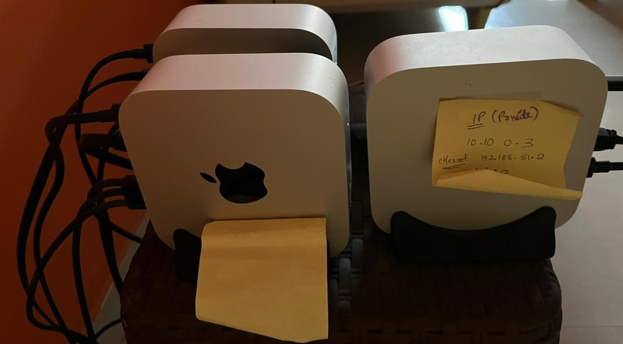 My Mac Mini cluster - Thunderbolt setup guide.
Six Small MoE Models × Two Backends: llama.cpp vs MLX-LM on Apple Silicon
Platform: Mac Mini M4 16GB
CPU: 10-core Apple M4 · GPU: 10-core Apple M4 (Metal) · Neural Engine: 16-core (not used by either backend)
Memory: 16 GB unified LPDDR5 shared CPU+GPU+ANE · OS: macOS Sequoia
Backends: llama.cpp (Metal, -ngl 99 --parallel 1 -fa 1 --ignore-eos --no-cache-prompt --cache-ram 0) · MLX-LM (mlx_lm.server, 4-bit, --prompt-cache-size 0 --decode-concurrency 1)
Runs: llama.cpp - full sweep, 6 models. MLX-LM - 3 models (2 have no published 4-bit MLX conversion or fail to load; see caveats below)
Sweep: prompt ∈ {256, 512, 1024, 2048, 4096, 30720} tok × gen ∈ {256, 512, 1024} tok × 20 reqs/combo
Concurrency: 1 (single-user)
Canonical cell: ctx=30720, gen=1024 - the longest-context, longest-generation point in the sweep, cited throughout as its exemplar endpoint rather than as the headline result
Key metric: output tok/J = OSL ÷ (decode_power_W × p50_decode_s) - decode-phase energy only
Raw data: full per-cell JSON exports (profile_export_aiperf.json + powermetrics.log + server logs) live in the smolbenchmark artifacts directory - no external dataset was published for this run.
Table S.1 lists the artifact coverage used throughout this report.
Table S.1: Benchmark artifact coverage by backend
| Backend | Artifact dir | Models | Cells |
|---|---|---|---|
| llama.cpp | artifacts/mac-m4-moe-20260704-0115/llamacpp |
6 | 108 |
| MLX-LM | artifacts/mac-m4-moe-20260712-1733/mlxlm |
3 | 54 |
Github for scripts, code, and the plotting notebooks that generated every chart below: smolbenchmark / mixture-of-experts.
Backend coverage caveat:
smallthinker-4b-a0.6bhas no published 4-bit MLX conversion, so it only has llama.cpp data.gemma4-e2b/gemma4-e4bare natively multimodal (text + vision + audio tower weights) - every MLX conversion (unsloth and mlx-community) keeps the full VLM-nested structure thatmlx_lm.servercannot load (it needsmlx_vlm.serverinstead), so both fail MLX-LM’s smoke test. Comparing llama.cpp against a different serving stack for those two would not be a fair backend comparison, so no MLX-LM data exists for them.
Executive Summary
Six small MoE / hybrid-MoE models were benchmarked on Mac Mini M4 under llama.cpp (Metal), and the three with published 4-bit MLX weights were also benchmarked under MLX-LM, for a direct backend comparison. Each model ran 18 combinations of prompt × generation length (20 requests per combo) spanning ctx=256 to a 30,720-token cell - so every claim below describes the whole sweep, with the long-context cell used as the exemplar endpoint rather than the headline result.
Key finding (full sweep): the model ranking is context-dependent. Across the sweep the models do not hold their order. SmallThinker-4B-A0.6B is the clear leader at the short-context end (126.42 tok/s at ctx=256, gen=1024), but it retains only 43.5 % of that by the long-context end (55.0 tok/s) - the steepest decay of any model tested. LFM2.5-8B-A1B starts slower (83.0 tok/s at ctx=256, gen=1024) but retains 76.7 % across the same span, so it overtakes SmallThinker somewhere between ctx=4096 and ctx=30720. “Fastest model” is a property of the context length, not of the model.
Backend finding (full sweep) - MLX vs llama.cpp:
-
llama.cpp vs MLX-LM is architecture-dependent, not a clean sweep either way. Granite-4.0-H-Tiny is consistently faster under MLX-LM across the whole sweep; Trinity-Nano-Preview and LFM2.5-8B-A1B are marginally faster under llama.cpp.
-
There is no single “winning” backend for this model class on Apple Silicon - unlike the CUDA/Jetson case where llama.cpp swept almost every model.
Efficiency across the sweep:
- SmallThinker-4B-A0.6B holds the best tok/J cell anywhere in the sweep (8.97 tok/J at ctx=512, gen=1024) and the best short-context throughput (130.75 tok/s), at ~3.6 GB peak RSS under Q4_K_M
- Trinity-Nano-Preview is 2nd-best on tok/J anywhere in the sweep (6.98 at ctx=512, gen=1024), in the smallest footprint (~4.3 GB peak RSS)
The long-context end of the sweep (ctx=30720, gen=1024 - the canonical cell), llama.cpp:
- LFM2.5-8B-A1B leads on throughput (63.73 tok/s, 4 % ahead of Trinity-Nano, 16 % ahead of SmallThinker)
- Trinity-Nano-Preview edges ahead on decode tok/J (4.6884 vs LFM2.5’s 4.5605) because its decode power is markedly lower (13.04 W vs 14.01 W), more than offsetting LFM2.5’s throughput lead
The sweep’s longest-context cell is tabulated in Table 1 for llama.cpp and Table 2 for MLX-LM. All other results in this report are quoted across the sweep; use Figure 1 and Figure 3 for the full curves.
Table 1: Throughput and efficiency at the long-context end of the sweep (ctx=30720, gen=1024 - the canonical cell) - llama.cpp, all 6 models
| Model | Total Params | Active Params | Output Tok/s | Output Tok/J | Peak RAM (MB) |
|——-|——–:|——–:|————-:|————-:|————-:|
| lfm2.5-8b-a1b | 8.3B | 1.5B | 63.73 | 4.5605 | 5473 |
| trinity-nano | 6B | 1B | 61.08 | 4.6884 | 4543 |
| smallthinker-4b-a0.6b | 4B | 0.6B | 55.04 | 3.8847 | 3716 |
| granite4-h-tiny | 7B | 1B | 45.45 | 3.0197 | 4706 |
| gemma4-e2b | 5.1B | 2.3B | 42.04 | 2.6039 | 3448 |
| gemma4-e4b | 8B | 4.5B | 22.53 | 1.4756 | 5592 |
Why is
trinity-nanoperforming better thangranite4-h-tinyin terms of decode tok/J? At this celltrinity-nanoboth decodes faster (61.08 vs 45.45 tok/s) and at lower decode power (13.04 W vs 15.07 W), so it wins on both terms of the ratio.
Table 2: Same cell under MLX-LM (3 models with published MLX weights)
| Model | Total Params | Active Params | Output Tok/s |
Output Tok/J |
Peak RAM (MB) |
|---|---|---|---|---|---|
| granite4-h-tiny | 7B | 1B | 59.41 | 5.4884 | 3683 |
| trinity-nano | 6B | 1B | 55.11 | 4.6413 | 3712 |
| lfm2.5-8b-a1b | 8.3B | 1.5B | 54.99 | 3.8666 | 4500 |
1. Test Setup
1.1 Hardware
The benchmark host is specified in Table 3.
Table 3: Hardware configuration
| Component | Detail |
|---|---|
| Board | Mac Mini M4 (Apple Silicon Desktop) |
| CPU | Apple M4, 10-core |
| GPU | Apple M4, 10-core, Metal 3 |
| Neural Engine | 16-core (unused by either backend under test) |
| Memory | 16 GB unified LPDDR5, shared CPU + GPU + ANE |
| Storage | NVMe SSD |
| Cooling | Active (internal fan); no throttling observed in any run (see Thermal Summary) |
1.2 Software Stack
The exact runtime versions and launch details are listed in Table 4.
| Layer | Version / Detail |
|---|---|
| Board | Mac Mini M4 16 GB |
| OS | macOS Sequoia |
| llama.cpp | Version 9730 (e475fa2b5); Metal backend, built with -DGGML_METAL=ON, -ngl 99 --parallel 1 -c <ctx> -t 1 -fa 1 --prio 2 --mlock --ignore-eos --no-cache-prompt --cache-ram 0 |
| MLX-LM | MLX-LM 0.31.3 with MLX 0.32.0; mlx_lm.server, 4-bit MLX weights, --prompt-cache-size 0 --decode-concurrency 1 --prompt-concurrency 1 |
| Load generator | aiperf (NVIDIA AI Performance tool), synthetic prompts at exact target token counts |
| Requests per combo | 20 requests, single run per combo - each model × prompt × gen cell was measured once (no repeat runs); the only repetition is the 20 requests within a combo |
| Power telemetry | powermetrics --samplers cpu_power,gpu_power,thermal -i 50, Combined (CPU+GPU+ANE) rail |
| RAM telemetry | ps -o rss= on the server PID, sampled every 50 ms; report uses the peak |
| Python | pandas, seaborn, matplotlib for chart generation |
| Concurrency | 1 user, 1 request at a time (--parallel 1 / --decode-concurrency 1) - single-user latency and throughput profile only |
| Context size | 32768 (max_prompt(30720) + max_gen(1024) + 1024 headroom) |
Flag parity note: llama.cpp’s
--ignore-eosforces exactlygenoutput tokens every request. MLX-LM’s server has no equivalent flag - it stops at EOS whenever the model emits one, which is the source of the OSL-mismatch caveat in section 4.3.
1.3 Models Under Test
| Model | Quant | Total Params | Active Params† | Peak RSS @ ctx=256 (MB) | Architecture‡ |
|---|---|---|---|---|---|
| SmallThinker-4B-A0.6B | Q4_K_M | 4B | 0.6B | 3644 | Standard Transformer MoE (32 experts, top-4) |
| Trinity-Nano-Preview | Q4_K_M | 6B | 1B | 4338 | Standard Transformer MoE (128 experts, top-8 + 1 shared) |
| Granite-4.0-H-Tiny | Q4_K_M | 7B | 1B | 4581 | Hybrid Mamba-2 + Transformer MoE (64 experts, top-6; 36 Mamba / 4 attention layers) |
| LFM2.5-8B-A1B | Q4_K_M | 8.3B | 1.5B | 5428 | Hybrid Conv + Attention MoE (32 experts, top-4; alternating conv/attention layers) |
| Gemma-4-E2B-it | Q4_K_M | 5.1B | 2.3B | 3377 | Dense elastic (MatFormer + Per-Layer Embeddings) - not MoE |
| Gemma-4-E4B-it | Q4_K_M | 8B | 4.5B | 5558 | Dense elastic (MatFormer + Per-Layer Embeddings) - not MoE |
Disclaimer: Gemma-4-E2B/E4B are not MoE - they’re included purely as a dense-model comparison point against the four actual MoE/hybrid-MoE models in this suite.
Quantization note: every model runs Q4_K_M (4-bit K-quant medium) under llama.cpp; MLX-LM runs the equivalent published 4-bit MLX conversion where one exists.
1.4 Benchmark Methodology
- For each
model×prompt×gencombo,aiperfsends 20 single-concurrency requests with synthetic prompts at the exact target token count. - Power is computed from
powermetrics’ Combined (CPU+GPU+ANE) rail (mW → W), sampled with-i 50(≈56 ms achieved). Per-request nanosecond timestamps fromprofile_export.jsonl(request_start_ns,request_end_ns) plus each request’s measuredtime_to_first_tokenclassify everypowermetricssample as prefill (request_start_ns→ first output token, i.e.request_start_ns+ TTFT) or decode (first output token →request_end_ns).request_ack_nsis deliberately not used as the phase boundary: it is the HTTP acknowledgement (~10 ms in), not the arrival of the first decoded token, so it would collapse the prefill window to ~0 samples and fold the whole TTFT into the decode window. Onepowermetricsquirk matters here: each sample block is stamped with a whole-second wall clock, so at ~56 ms cadence roughly 18 consecutive samples share a single timestamp. Classifying those directly against sub-second phase windows would drag whole seconds of decode power into the short prefill windows (at ctx=256 the prefill window is only ~0.25 s length), flattening prefill power toward decode power and inflating short-context prefill efficiency by up to ~40 %. The per-block(56.75ms elapsed)field is an exact clock - summing it reproduces the run duration to under a second - so sample times are rebuilt to ~56 ms resolution by accumulating it and solving for the one free sub-second phase before classification (Appendix I.6).decode_power_Wis the median of samples inside decode windows;p50_decode_sis the median per-request decode duration.output_tok_J=OSL÷ (decode_power_W×p50_decode_s) - decode-phase energy only, so the high-power prefill spike doesn’t inflate the denominator. - Each server was launched once per model, smoke-tested, then swept through all 18 combos before restart for the next model.
--no-cache-prompt --cache-ram 0(llama.cpp) /--prompt-cache-size 0(MLX-LM) disable KV-cache reuse across requests so prefill cost isn’t unfairly cheap on repeated synthetic prompts. This specifically protects the variance within a combo’s 20 repeated requests (--synthetic-input-tokens-stddev 0, same target length, different random content, same live server): without it, a later request could get a partial or full prefill discount from an earlier one’s cached prefix, understating that request’s true TTFT/prefill cost and skewing the p50/p90/p99 spread reported for the combo. It has nothing to do with variance between combos - those already differ by prompt length, so there’s no caching concern there. - Latency percentile used throughout: all
TTFT,ITL, and request latency (RL) values reported in charts, tables, and energy calculations use the p50 (median) over the 20 requests per combo, to avoid inflation from occasional slow requests (GC pause, OS scheduling). p90 and p99 are available inreport.mdfor tail-latency analysis. - RSS sampling captures the server process’s resident memory every 50 ms during each combo; the report keeps the peak - this is model weights + KV-cache + activation footprint at that specific prompt/gen length, not a fixed “model size.”
- Run-start warm-up is excluded from all power-derived statistics. The first combo of each model/backend run (
gen=256/ctx=256;gen=256/ctx=512for MLX-LM Trinity, whose ctx=256 cell did not run) is measured while the SoC is still in its post-model-load high-power state: thepowermetricsCombined rail runs ~1-2 W above steady state and only decays over ~40-95 s, so for the shortest combos the whole combo is inflated. That single cell is voided from total/prefill/decode power and thetok/Jfamily so it cannot masquerade as a short-context effect; throughput, TTFT/ITL/RL and RSS keep all available combos.
2. Results: Charts
All charts below plot both backends together: llama.cpp (all 6 models) and MLX-LM (the 3 shared models — see backend caveats) are overlaid on the same axes wherever the metric allows it. Every model label in every chart (legend, axis, or heatmap title) is suffixed with its (total params B=active params B) from Table 5 - e.g. granite4-h-tiny (7B=1B) - so parameter scale is visible without cross-referencing the table.
2.1 Throughput vs Prompt Length
Figure 1 plots output tok/s and prefill tok/s by model across all 3 generation lengths (one row per gen, gen=256/512/1024), llama.cpp (solid) vs MLX-LM (dashed). Throughput falls monotonically as context grows, but not at the same rate:
Figure 1: Throughput - output tok/s and prefill tok/s vs prompt length, all models, all 3 generation lengths (gen=256/512/1024), llama.cpp (solid) vs MLX-LM (dashed)
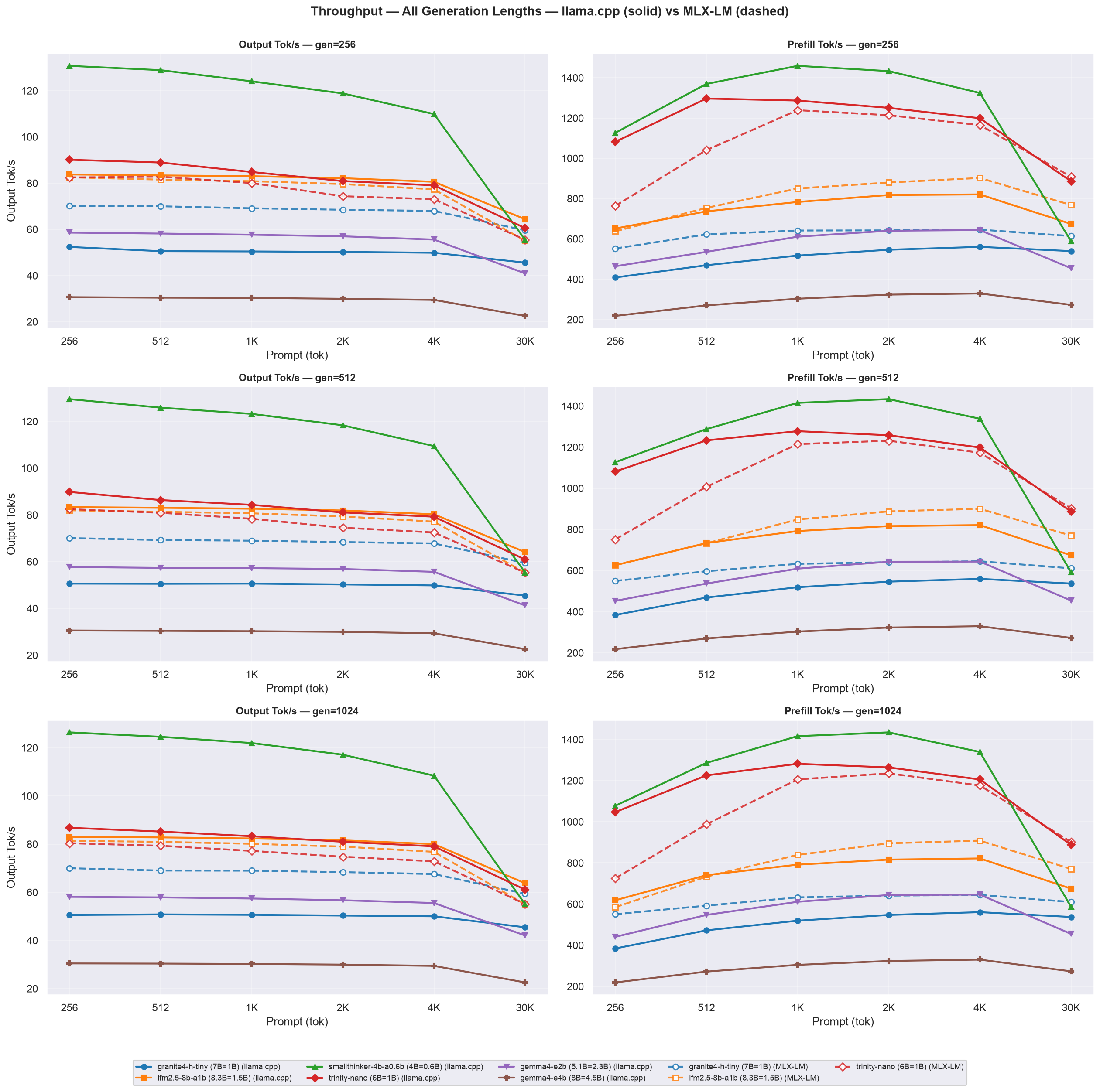
Granite-4.0-H-TinyandTrinity-Nano-Previeware the two models with 1B active parameters, and yet their output tok/s and prefill tok/s - the two columns of Figure 1, generated and input tokens per second respectively, Appendix I.1 - both differ by an appreciable margin, up untill 30k ctx length where the Mamba arch shines. One is a hybrid Mamba-2 + Transformer MoE design while other is standard transformer MoE. The reason for the gap could be in the design choice of their kernels.
Figure 1’s right-hand column is prefill tok/s (input tokens processed per second during the prompt phase) - a prompt-phase metric that is effectively independent of generation length (verified <1 % spread across gen at fixed ctx), so its three gen rows are near-identical.
Why Granite-4.0-H-Tiny prefills slower than Trinity-Nano-Preview at the same 1B active parameters.
- Counting MACs per token from each model’s config:
Per-token component Granite @ 256 Granite @ 30,720 Trinity @ 256 Trinity @ 30,720 Mamba projections + scan 540.6M 540.6M - - Attention (42 sliding + 14 global / 4 global) 28.3M 402.7M 176.1M 1203.8M MoE routing + experts 758.9M 758.9M 403.7M 403.7M Total 1327.8M 1702.1M 579.9M 1607.5M Granite ÷ Trinity 2.29× 1.06×
- At ctx=256 Granite does 2.29× the arithmetic per token while llama.cpp observes 2.73× its prefill time - at short context the gap is the FLOP gap.
- At ctx=30720 Trinity’s 14
full_attentionlayers go quadratic (~918M MACs/token) and the two converge to 1.06× on arithmetic - yet Granite is still ~1.6× slower (Figure 1).- Arithmetic alone does not explain that residual - the remaining gap is consistent with kernel efficiency: Granite’s prefill is a chain of modest-size ops (conv → scan → gate → elementwise), while Trinity’s is dominated by large attention GEMMs.
MACs =
d_in × d_outper linear;2 × n_heads × T_attended × head_dimper attention block, whereT_attended = min(ctx, sliding_window)on sliding layers andctxelsewhere;d_inner × d_stateper Mamba scan per token. Dimension counts are read from each model’s publishedconfig.json; norms, embeddings and router overhead are excluded, so these are relative magnitudes rather than absolute timings.
Figure 2 collects the section’s two throughput metrics into one picture: the best output tok/s and the best prefill tok/s each model reaches anywhere in its 18-combo sweep (solid bar = llama.cpp, hatched = MLX-LM), with the winning ctx/gen cell labelled under each bar; the per-model median across all 18 combos is tabulated in Table 6:
Figure 2: Best output tok/s and prefill tok/s per model across all 18 combinations, llama.cpp (solid) vs MLX-LM (hatched)
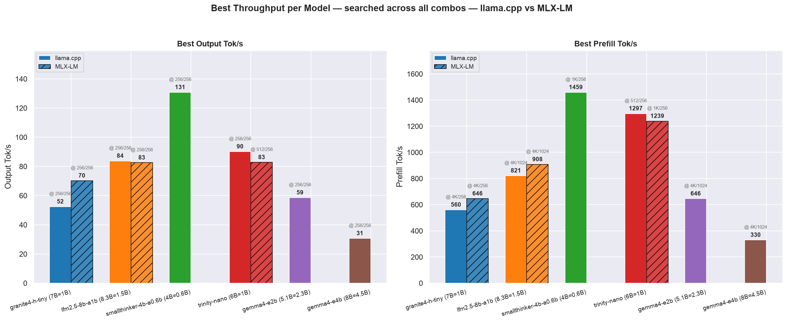
Every output-tok/s peak lands at ctx=256 or 512 - short-context throughput is the high-water mark for all six models, which is the retention story in 3.2 seen from the other end. The fastest cell for a model is not always its most efficient one (see 3.1).
- Unlike output tok/s, the best prefill tok/s cell is not pinned to the shortest context - prefill speed peaks at partway ctx for most models, consistent with the mid-sweep hump in Figure 1’s right-hand column. The two panels together are the “best case” envelope of the section: generation is fastest at short context, prefill is fastest in the middle.
Table 6: Median across all 18 combos - throughput, per model and backend (llama.cpp vs MLX-LM)
| Model | Total Params | Active Params | Output tok/s llama.cpp | Output tok/s MLX-LM | Prefill tok/s llama.cpp | Prefill tok/s MLX-LM |
|---|---|---|---|---|---|---|
| gemma4-e4b | 8B | 4.5B | 30.10 | - | 287.80 | - |
| gemma4-e2b | 5.1B | 2.3B | 57.10 | - | 577.96 | - |
| granite4-h-tiny | 7B | 1B | 50.37 | 68.71 | 527.91 | 627.12 |
| lfm2.5-8b-a1b | 8.3B | 1.5B | 82.24 | 79.86 | 761.59 | 804.37 |
| smallthinker-4b-a0.6b | 4B | 0.6B | 120.41 | - | 1331.19 | - |
| trinity-nano | 6B | 1B | 82.16 | 75.97 | 1215.08 | 1102.70 |
The median across all 18 combos is the typical cell for each model - read it against the best-cell bars in Figure 2. The two metrics rank differently: SmallThinker leads on output tok/s under llama.cpp, but LFM2.5 leads on prefill tok/s.
2.2 Energy Efficiency
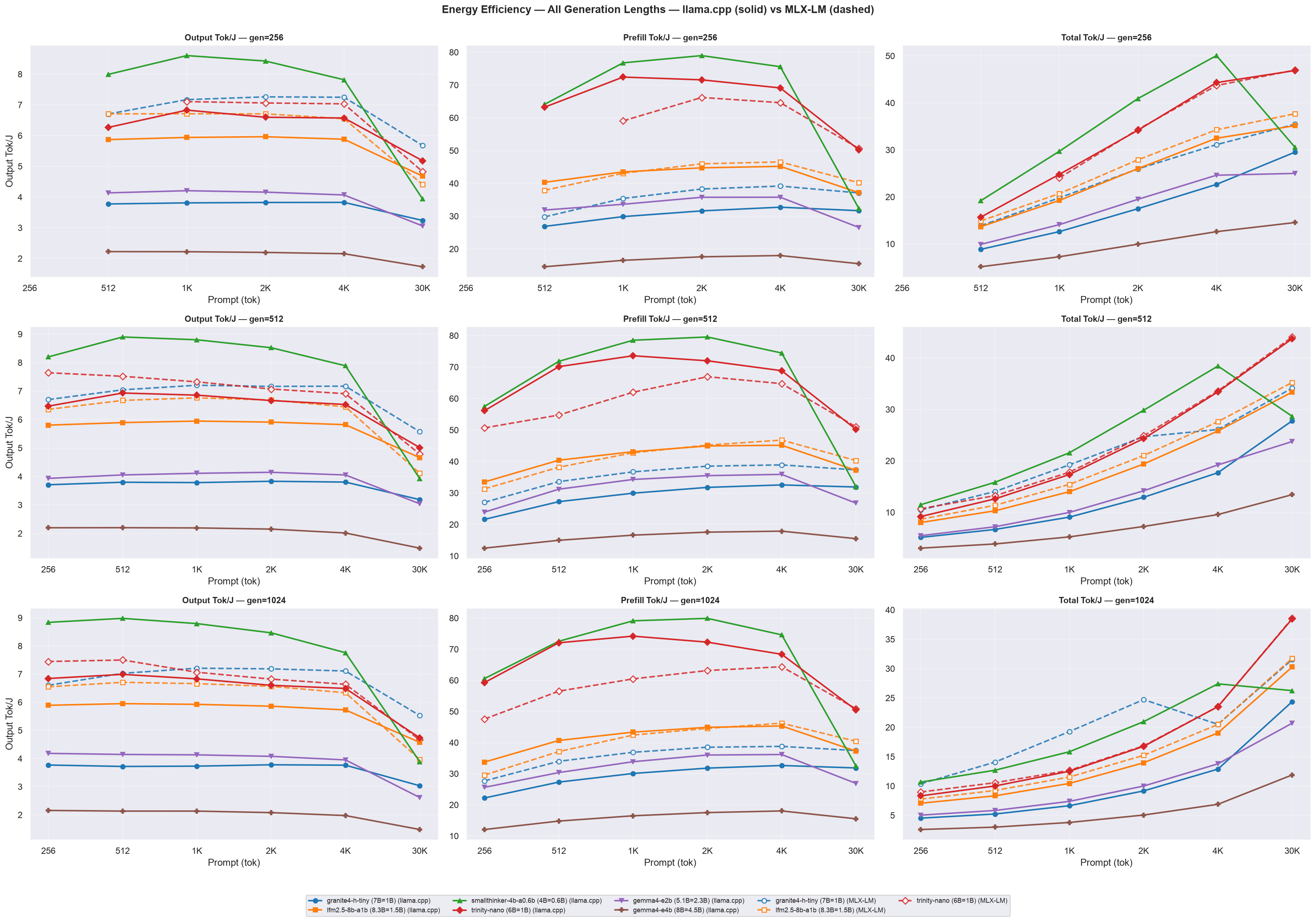
- Figure 3 plots the three efficiency phases - output tok/J, prefill tok/J and total tok/J - by model across all 3 generation lengths (one row per gen), llama.cpp (solid) vs MLX-LM (dashed). Every model’s output tok/J decays with context length as decode power creeps up and per-token throughput drops, while total tok/J rises (input tokens are ~10× cheaper than output tokens). The middle column, prefill tok/J, is not monotonically falling: it starts at its lowest point at ctx=256 (the phase clock is shortest there, so the fixed per-request dispatch overhead eats the largest share of the prefill window), rises to a peak at ctx≈2048-4096, then eases back at the 30,720-token end as the growing attention cost starts to bite:
Figure 3: Energy efficiency - output tok/J, prefill tok/J and total tok/J vs prompt length, all models, all 3 generation lengths (gen=256/512/1024), llama.cpp (solid) vs MLX-LM (dashed)
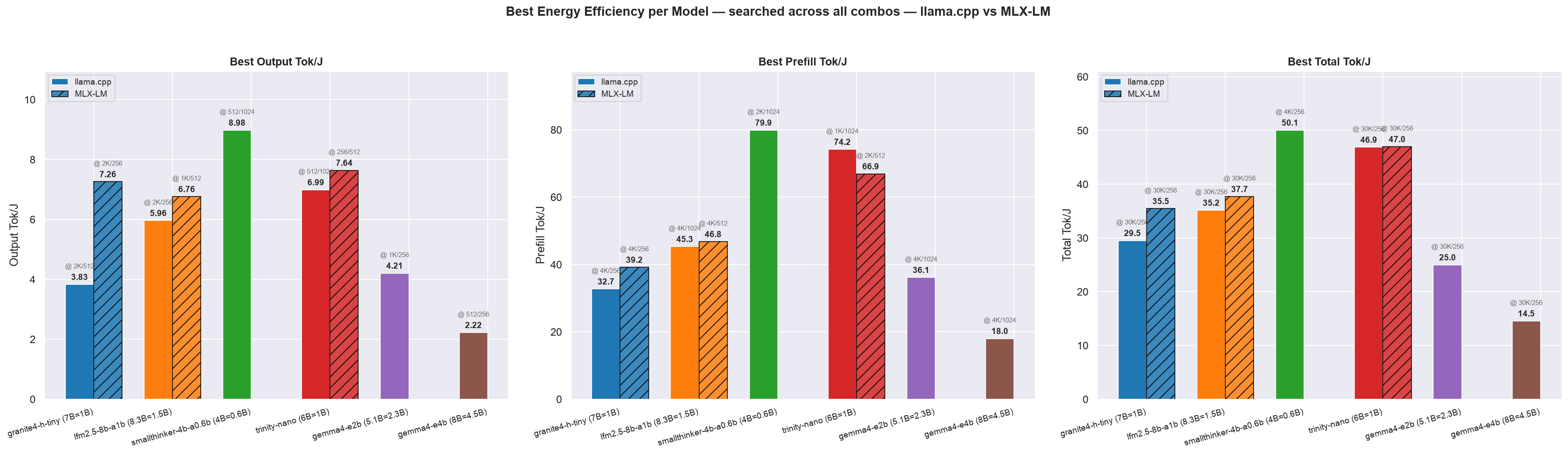
- Figure 4 collects all three of the section’s efficiency metrics into one picture: the best output tok/J, prefill tok/J and total tok/J per model, each searched across the sweep and both backends (solid bar = llama.cpp, hatched bar = MLX-LM). Each bar is labeled with the winning
ctx/gencell (e.g.@ 256/1024= ctx=256, gen=1024) so the source combo isn’t hidden; the per-model median across the sweep (power-derived, so the run’s first cell is excluded - §1.4) is tabulated in Table 7:
Figure 4: Best output tok/J, prefill tok/J and total tok/J per model across the sweep (power-derived; the run’s first cell is excluded as warm-up, §1.4), llama.cpp (solid) vs MLX-LM (hatched)
- Figure 3’s middle and right columns are prefill tok/J (input tokens per joule of prefill energy) and total tok/J ((input + output) tokens per joule of total request energy).
- Total tok/J grows with context - the opposite of Figure 3’s decode-only output tok/J - because input tokens are ~10× cheaper to process than output tokens are to generate.
- “Total” means the whole request: energy is
prefill_J+decode_Jand the token count isISL + OSL- a request both reads the prompt (ISL, paid in prefill_J) and writes the completion (OSL, paid in decode_J), so both phases must count.
Table 7: Median across the sweep - energy efficiency, per model and backend (llama.cpp vs MLX-LM); run’s first cell excluded as warm-up (§1.4)
| Model | Total Params | Active Params | Output tok/J llama.cpp | Output tok/J MLX-LM | Prefill tok/J llama.cpp | Prefill tok/J MLX-LM | Total tok/J llama.cpp | Total tok/J MLX-LM |
|---|---|---|---|---|---|---|---|---|
| gemma4-e4b | 8B | 4.5B | 2.15 | - | 16.46 | - | 6.87 | - |
| gemma4-e2b | 5.1B | 2.3B | 4.08 | - | 33.62 | - | 13.77 | - |
| granite4-h-tiny | 7B | 1B | 3.77 | 7.11 | 31.60 | 37.07 | 12.61 | 20.50 |
| lfm2.5-8b-a1b | 8.3B | 1.5B | 5.88 | 6.56 | 43.11 | 42.40 | 19.03 | 20.48 |
| smallthinker-4b-a0.6b | 4B | 0.6B | 8.43 | - | 74.45 | - | 26.24 | - |
| trinity-nano | 6B | 1B | 6.60 | 7.06 | 69.11 | 59.75 | 23.52 | 23.77 |
The same comparison as Table 6, for the three efficiency metrics. The backend gap is widest on output tok/J for Granite (3.77 vs 7.11) and all but absent on prefill tok/J for LFM2.5 (43.11 vs 42.40). Under llama.cpp the ranking mirrors Table 6’s throughput story - SmallThinker leads output tok/J (8.43) and total tok/J (26.24), while LFM2.5 leads prefill tok/J (43.11) - a model can win one efficiency axis without winning the others, because the three metrics weight prefill and decode energy very differently.
2.3 Latency
Figure 5 shows the three latency signals - TTFT p50, ITL (inter-token latency) p50, and request latency (E2E) p50 - by model across all 3 generation lengths (one row per gen), llama.cpp (solid) vs MLX-LM (dashed). TTFT scales with prompt length and is the dominant cost at ctx=30720 (34-113 s depending on model); ITL is the per-token decode cost once prefill is excluded:
Figure 5: Latency - TTFT / ITL / request latency p50 vs prompt length, all models, all 3 generation lengths (gen=256/512/1024), llama.cpp (solid) vs MLX-LM (dashed)
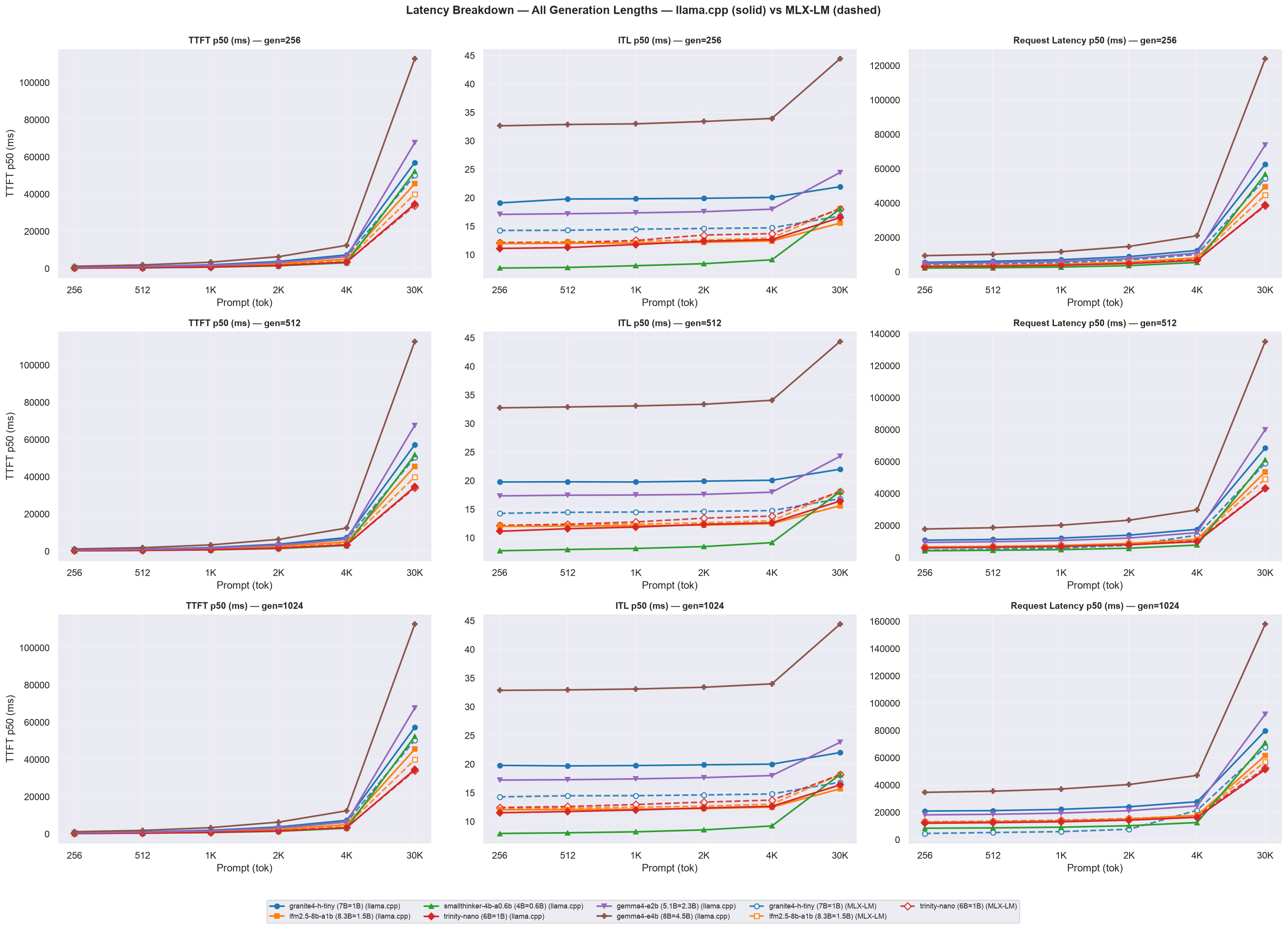
Figure 6 is the latency counterpart to Figure 2/Figure 4: each model’s fastest (minimum) TTFT, ITL and request latency anywhere in its 18-combo sweep, one panel per signal, with the winning ctx/gen cell labelled under each bar (solid bar = llama.cpp, hatched = MLX-LM); the per-model median across all 18 combos is tabulated in Table 8. Every best cell lands at ctx=256 - the mirror of Figure 2’s short-context throughput peaks.
Figure 6: Best TTFT / ITL / request latency per model across all 18 combinations (min), llama.cpp (solid) vs MLX-LM (hatched)
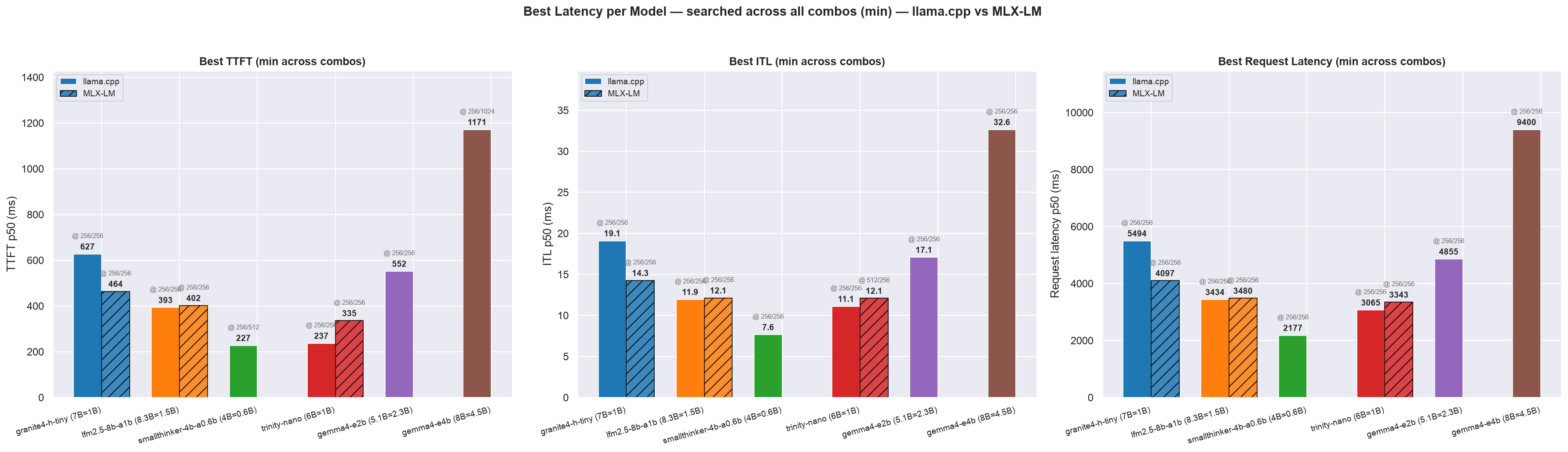
Table 8: Median across all 18 combos - latency p50, per model and backend (llama.cpp vs MLX-LM)
| Model | Total Params | Active Params | TTFT p50 (ms) llama.cpp | TTFT p50 (ms) MLX-LM | ITL p50 (ms) llama.cpp | ITL p50 (ms) MLX-LM | RL p50 (ms) llama.cpp | RL p50 (ms) MLX-LM |
|---|---|---|---|---|---|---|---|---|
| gemma4-e4b | 8B | 4.5B | 4859 | - | 33.23 | - | 26515 | - |
| gemma4-e2b | 5.1B | 2.3B | 2431 | - | 17.51 | - | 13810 | - |
| granite4-h-tiny | 7B | 1B | 2863 | 2405 | 19.85 | 14.55 | 15749 | 6376 |
| lfm2.5-8b-a1b | 8.3B | 1.5B | 1906 | 1755 | 12.16 | 12.52 | 10045 | 9945 |
| smallthinker-4b-a0.6b | 4B | 0.6B | 1076 | - | 8.31 | - | 6740 | - |
| trinity-nano | 6B | 1B | 1211 | 1254 | 12.17 | 13.17 | 8900 | 9513 |
The same comparison as Table 6/Table 7, for the three latency signals. TTFT dominates RL at the median cell (a long prompt is mostly prefill), which is why the backends separate far more on RL than on ITL.
2.4 Power Draw and Thermal Summary
Figure 7 compares total / prefill / decode power by model across all 3 generation lengths (one row per gen) for llama.cpp vs MLX-LM; Figure 8 condenses the sweep to one panel per power metric:
Figure 7: Power - total / prefill / decode power vs prompt length, all models, all 3 generation lengths (gen=256/512/1024), llama.cpp (solid) vs MLX-LM (dashed)
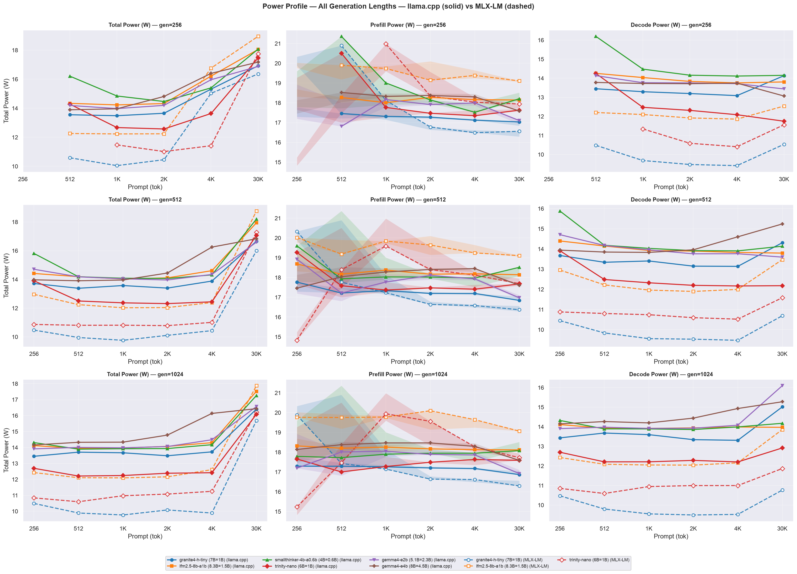
- The prefill column carries a translucent band - the min-max spread of prefill power across the three generation-length runs.
- The band is narrow where each prefill window (== TTFT) is long enough to hold hundreds of ~56 ms
powermetricssamples (≤0.5 W at ctx≥4096) and blows up to ~2-3.6 W at ctx=256/512, where a 0.2-0.7 s window holds only a handful of samples and the pooled median becomes sensitive to sub-sample phase alignment. Read the prefill column’s ordering as real only at ctx≥4096; at ctx=256/512 it is a sampling floor, not a gen-length effect.
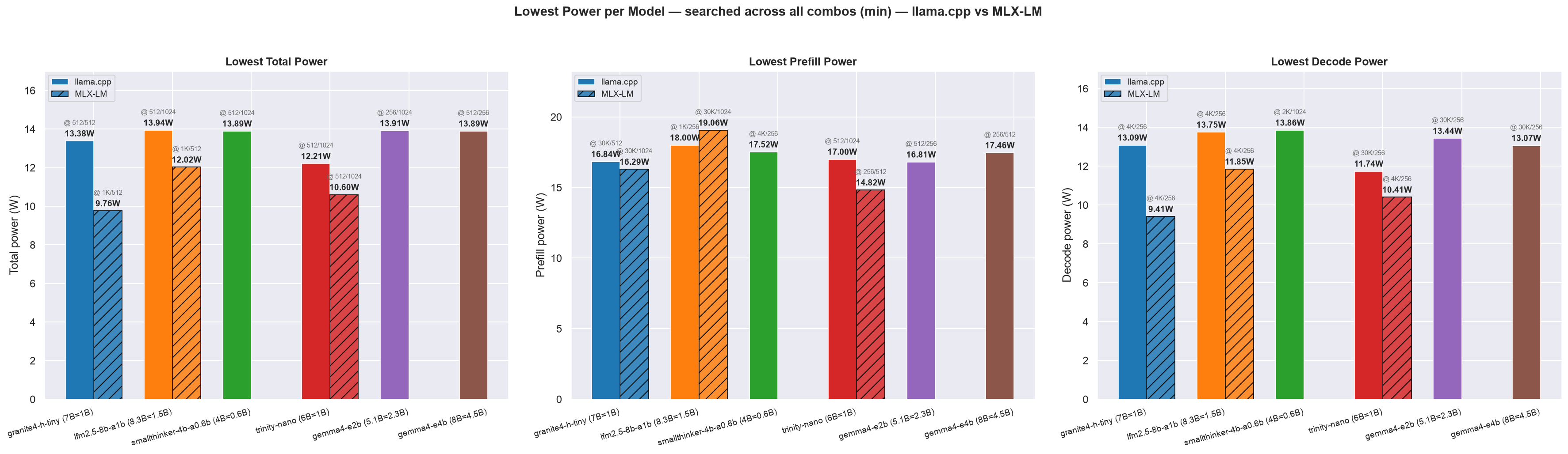
Figure 8 collects the section’s three power metrics into one picture - each model’s lowest total, prefill and decode power (Combined CPU+GPU+ANE) across its sweep (bar), with the winning ctx/gen cell labelled under each bar:
Figure 8: Lowest total / prefill / decode power per model across the sweep (the run’s first cell is excluded as warm-up, §1.4), llama.cpp (solid) vs MLX-LM (hatched)
macOS
powermetrics’thermalsampler on the M4 does not expose a per-core junction temperature the waytegrastatsdoes on Jetson, so no CPU/GPU °C columns are reported here - only the throttling flag, derived from whether decode throughput degraded mid-run. No model throttled at any point in either sweep.
Table 9: Power & thermal summary - median across the sweep, per model and backend (llama.cpp vs MLX-LM); run’s first cell excluded as warm-up (§1.4)
| Model | Total Params | Active Params | Median Total W llama.cpp | Median Total W MLX-LM | Throttled |
|---|---|---|---|---|---|
| gemma4-e4b | 8B | 4.5B | 14.44 | - | No |
| gemma4-e2b | 5.1B | 2.3B | 14.19 | - | No |
| granite4-h-tiny | 7B | 1B | 13.67 | 10.43 | No |
| lfm2.5-8b-a1b | 8.3B | 1.5B | 14.30 | 12.26 | No |
| smallthinker-4b-a0.6b | 4B | 0.6B | 14.31 | - | No |
| trinity-nano | 6B | 1B | 12.57 | 11.01 | No |
Table 9 gives each model’s median across the sweep of whole-combo total power (the run’s first cell is excluded as warm-up - §1.4) - the same estimator as the Total Power line in Figure 7. Two things stand out: under llama.cpp every model lands in a narrow 12.6-14.4 W band despite a ~7× spread in active parameters (0.6 B to 4.5 B), and MLX-LM draws noticeably less for the same three models (10.4-12.3 W vs 12.6-14.4 W) - consistent with MLX being a purpose-built Apple Silicon framework with less server-side overhead than the cross-platform Metal backend. No model throttled anywhere in either sweep.
2.5 GPU Usage
powermetrics’ own GPU-usage section (GPU HW active frequency, GPU HW active residency) is a signal none of the tok/s, tok/J, or power charts above use directly - it says how hard the Metal GPU itself is working, independent of how many output tokens that work produces.
Figure 9: GPU frequency and residency vs prefill / decode power - all cells (all gen × ctx, both backends); each segment runs prefill → decode for one cell
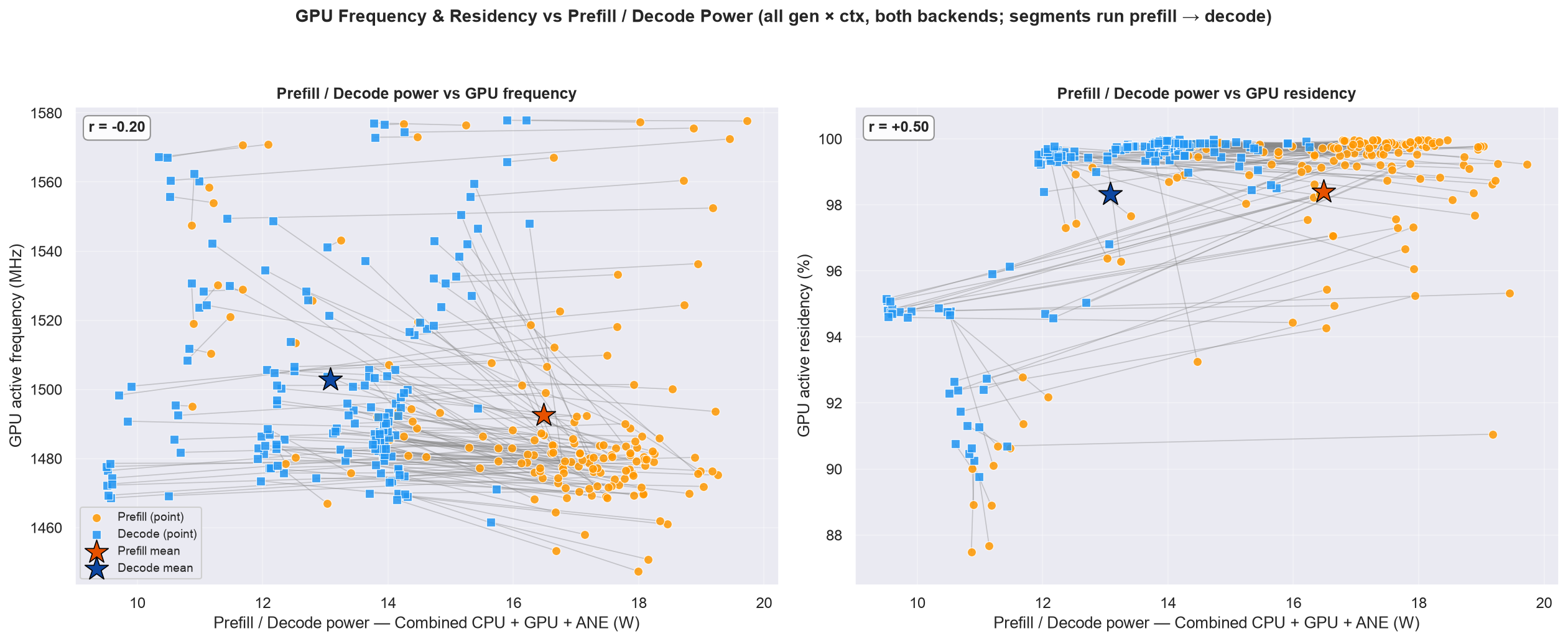
Prefill and decode are not the same workload, so they can sit at (near-)the same >GPU clock while drawing very different power - power is energy per cycle × >cycles per second, and the two phases differ sharply in the first term:
- Prefill cycle: ALUs switching, doing multiplies → high $E_{cyc}$.
- Decode cycle: units mostly stalled on LPDDR5, little switching → low >$E_{cyc}$.
So for two different phases:
Phase $E_{cyc}$ $f$ (MHz) $P = E_{cyc} \times f$ Prefill high (~2×) 1477 17-18 W Decode low 1550 12-15 W
Figure 9b: GPU active clock as a distribution - prefill vs decode vs prompt length, all 3 generation lengths (gen=256/512/1024); models pooled into one split violin per cell (llama.cpp left / MLX-LM right); dotted lines mark the two hardware-chosen p-states
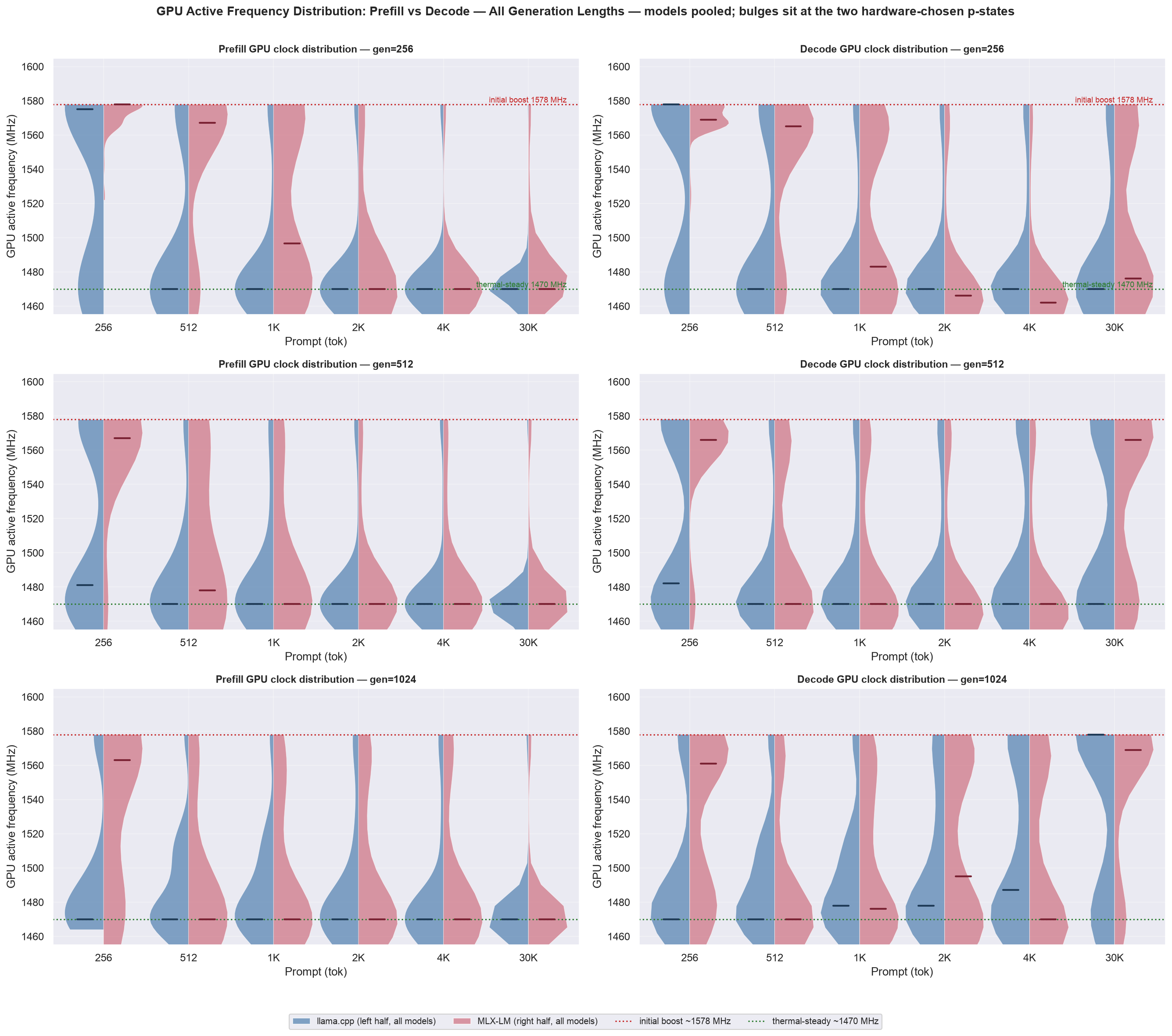
- The clock is bimodal (~1578 MHz initial-boost → ~1470 MHz thermal-steady); a cell mean is just the duty-cycle mix of those two, which is why it shifts with run length. The bulges sit on the two dotted rails; prefill sits lower than decode and the gap grows with context (~3 MHz at ctx=256 → 15-83 MHz at ctx=30720 under llama.cpp) - opposite of “prefill should clock highest”. Likely the governor trading clock against prefill’s higher sustained power (17-18 W vs decode’s 12-15 W, Figure 7); Figure 9d shows the shape.
- The clock band is narrow (~1450-1578 MHz) while output tok/s varies several-fold (Figure 1), so throughput differences come from work per token, not from the GPU clocking differently. MLX-LM’s right half tracks llama.cpp’s left - hardware/OS behaviour, not a backend property.
Figure 9c: GPU active residency - prefill vs decode vs prompt length, all models, all 3 generation lengths (gen=256/512/1024), llama.cpp (solid) vs MLX-LM (dashed); the two columns share one y-range
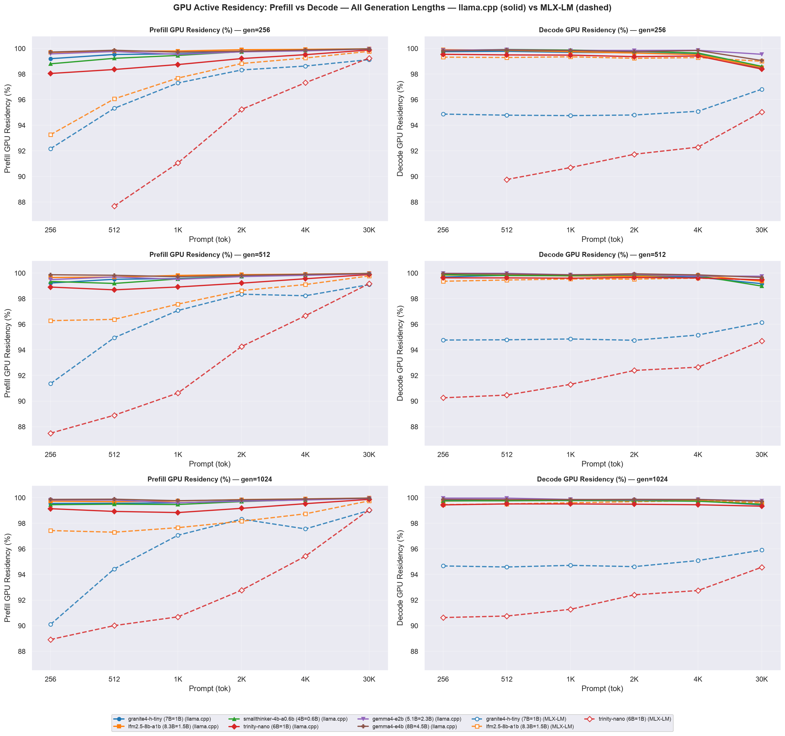
- Both phases sit ~99.5-100 % resident at mid/long context; the real signal is a crossover - decode is marginally more resident at short context, then prefill takes over by ~ctx=4096 (~99.9 % vs decode’s ~99.4 %). Residency counts engagement, not useful work: whole-combo residency rises with context while output tok/s falls (I.14).
- MLX-LM’s decode residency drops to 94.6-95.9 % for Granite and Trinity (Table 10b) while its prefill stays ~99 % - the one clear backend difference in the GPU section, matching MLX-LM’s lower total power in Figure 8.
Figure 9d: GPU active frequency and residency, prefill vs decode - Granite-4.0-H-Tiny (llama.cpp), canonical combo (ctx=30720, gen=1024), first 4 of 20 requests
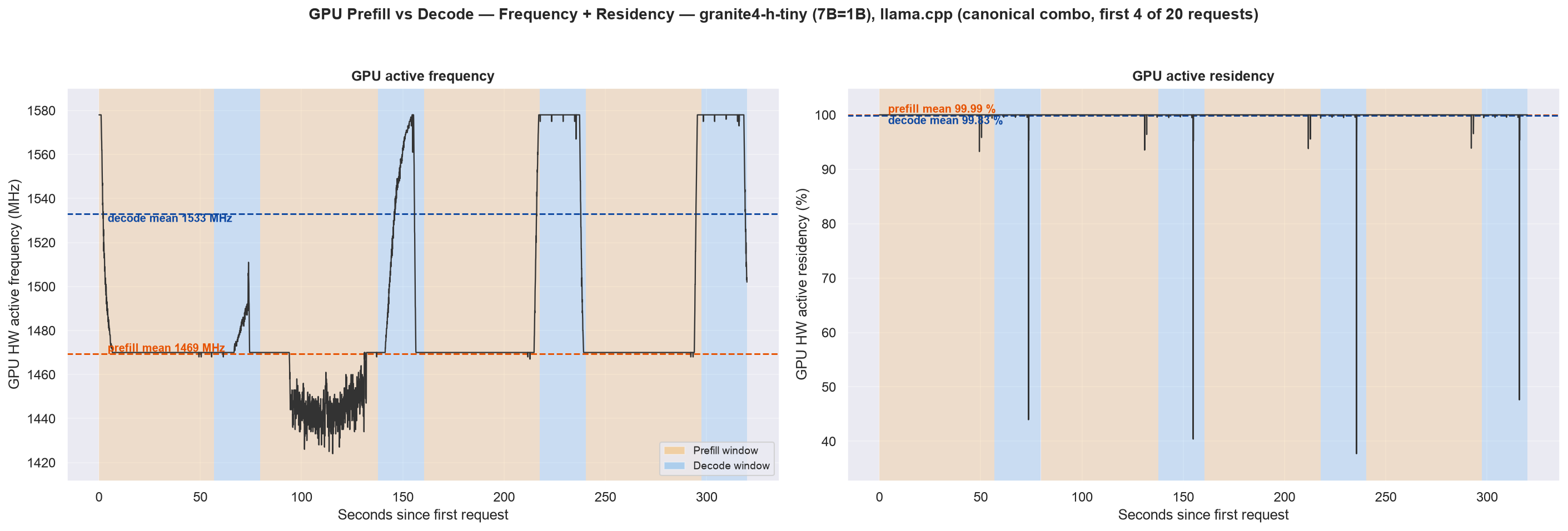
- Left panel: each request is one prefill plateau at ~1480 MHz (shaded orange) followed by a decode step up to ~1550 MHz (shaded blue), repeating for all 20 requests; the dashed lines mark each phase’s mean. Right panel: residency sits at ~99.8 % through prefill and ~99.4 % through decode, dipping briefly at each request→request hand-off.
- The clock does not ramp within prefill - the orange window is flat - and the sharp spike to the ~1578 MHz ceiling sits exactly at the prefill→decode hand-off. So the “climb to ~1570 MHz” that a whole-run view reads as prefill ramping up is that transition into decode, not the prefill itself.
Table 10 and Table 10b give the per-model canonical-cell active frequency and active residency, split by phase, that Figures 9-9d condense (terms defined in I.14).
Table 10: GPU utilization at the canonical cell (ctx=30720, gen=1024), by phase, llama.cpp
| Model | Total Params | Active Params | Prefill freq (MHz) | Decode freq (MHz) | Prefill residency (%) | Decode residency (%) |
|---|---|---|---|---|---|---|
| gemma4-e4b | 8B | 4.5B | 1477 | 1560 | 99.96 | 99.71 |
| gemma4-e2b | 5.1B | 2.3B | 1476 | 1548 | 99.94 | 99.76 |
| granite4-h-tiny | 7B | 1B | 1477 | 1551 | 99.96 | 99.43 |
| lfm2.5-8b-a1b | 8.3B | 1.5B | 1472 | 1487 | 99.97 | 99.49 |
| smallthinker-4b-a0.6b | 4B | 0.6B | 1447 | 1470 | 99.97 | 99.49 |
| trinity-nano | 6B | 1B | 1469 | 1537 | 99.87 | 99.34 |
Table 10b: GPU utilization at the canonical cell (ctx=30720, gen=1024), by phase, MLX-LM (3 shared models)
| Model | Total Params | Active Params | Prefill freq (MHz) | Decode freq (MHz) | Prefill residency (%) | Decode residency (%) |
|---|---|---|---|---|---|---|
| trinity-nano | 6B | 1B | 1481 | 1549 | 99.05 | 94.57 |
| lfm2.5-8b-a1b | 8.3B | 1.5B | 1476 | 1543 | 99.75 | 99.61 |
| granite4-h-tiny | 7B | 1B | 1479 | 1542 | 99.00 | 95.91 |
- Decode out-clocks prefill for every model, both backends, and the gap grows with context - from +0-3 MHz at ctx=256 to +15-83 MHz at ctx=30720 (LFM2.5 1472 → 1487, gemma4-e4b 1477 → 1560). Peak anywhere in the dataset is 1578 MHz; every canonical-cell average is within 8 % of that ceiling.
- Residency separates the backends in decode, not prefill. llama.cpp’s decode stays ≥ 99.3 % for all six models; MLX-LM’s drops to 94.6-95.9 % for Granite and Trinity while its prefill stays ~99 %.
2.6 Processor Usage and Frequency
The same powermetrics logs also report per-cluster CPU frequency and residency (E-Cluster - 6 efficiency cores - and P-Cluster - 4 performance cores - on the M4’s 10-core CPU; terms defined in I.14). This tells a very different story from the GPU: it shows where request scheduling / KV-cache bookkeeping actually runs, separate from the Metal-GPU matmuls charted above. Figure 10 charts residency across the full sweep and Figure 10b does the same for P-Cluster frequency, both backends - llama.cpp all 6 models (solid), MLX-LM the 3 shared models (dashed). The canonical combo is then kept as the exemplar endpoint in Figures 10c-10e.
Figure 10: E-Cluster vs P-Cluster active residency vs prompt length, all models, all 3 generation lengths (gen=256/512/1024), llama.cpp (solid) vs MLX-LM (dashed)
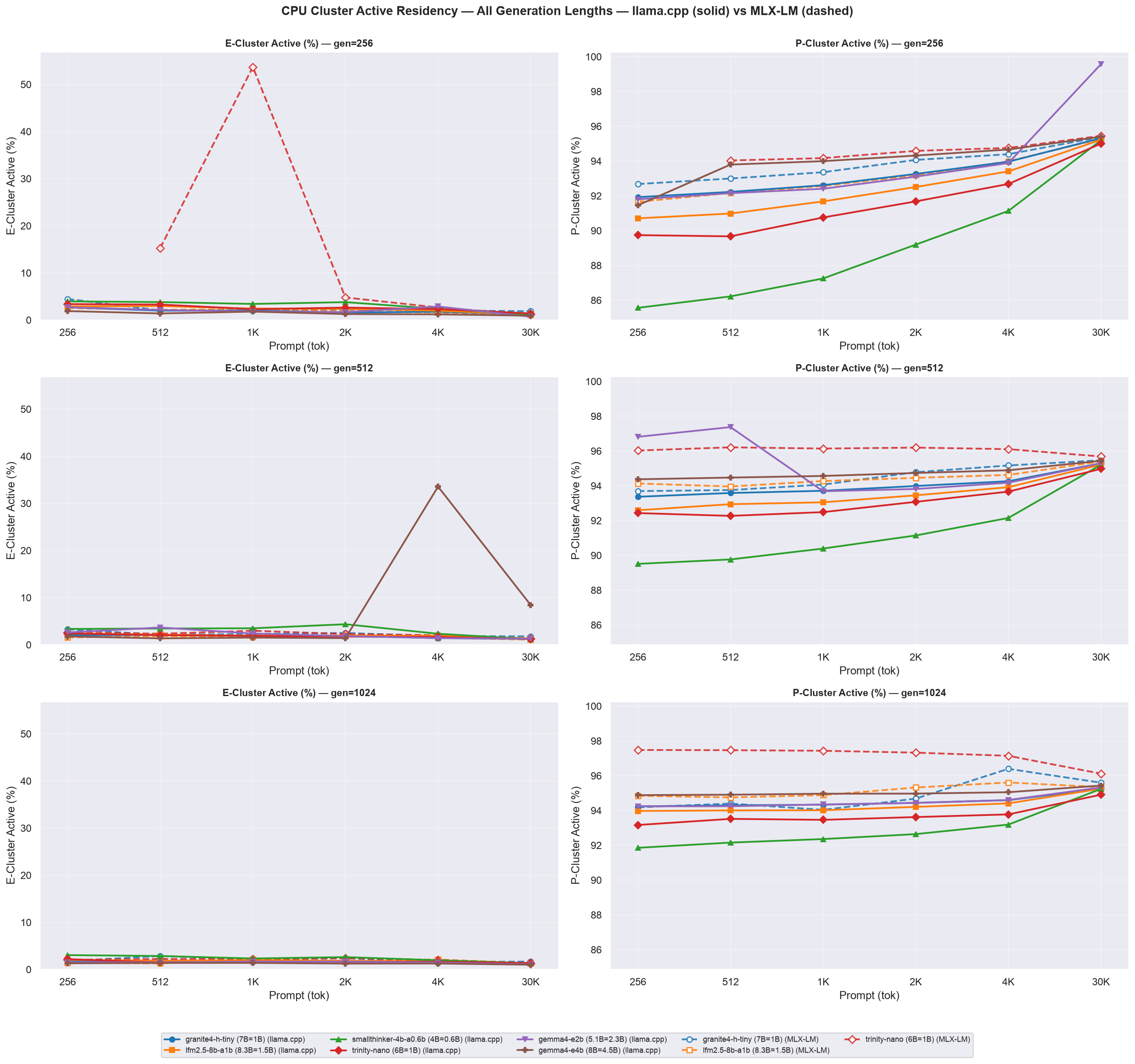
- Inference runs on the 4 performance cores across the entire sweep under both backends. P-Cluster residency rises with prompt length (85.6-97.5 % at ctx=256 → 94.9-99.6 % at ctx=30720) while the 6 efficiency cores stay near-idle (157 of 161 cells < 5 %). macOS keeps llama.cpp’s
-t 1loop and MLX-LM’s request handling on the P-cluster. - Same story as the GPU (2.5): once context is long, the busy resource is saturated (P-cluster 94.9-99.6 %, GPU 96.9-99.6 %) and the rest of the chip is untouched. Read the E-Cluster panel as “near-idle throughout”, not a per-model ranking.
Figure 10b: P-Cluster active frequency vs prompt length, all models, all 3 generation lengths (gen=256/512/1024), llama.cpp (solid) vs MLX-LM (dashed)
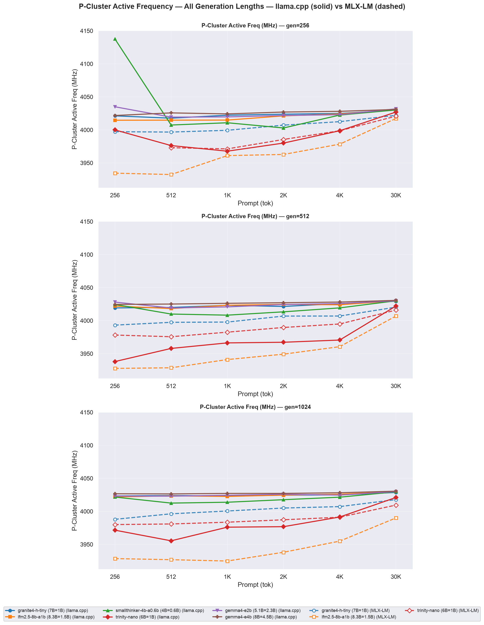
- The P-cluster is pinned near its maximum for every model at every cell in the sweep - the lines sit flat against the top of the axis, which is the finding: unlike Jetson’s
nvpmodelgovernor there is no CPU frequency stepping to observe here, not between requests, not prefill vs. decode, not across model sizes or backends. - The axis is zoomed to the measured band (~3.91-4.15 GHz) so the nine model/backend lines are individually visible rather than stacked in a sliver at the top of a 0-based panel. Even so the residual spread is tiny (3.93-4.14 GHz across the whole sweep) and the message is the absence of a governor, not a trend - Figure 10d keeps the 0-based bar view for contrast.
Figure 10c: E-Cluster vs P-Cluster active residency, llama.cpp vs MLX-LM, canonical combo
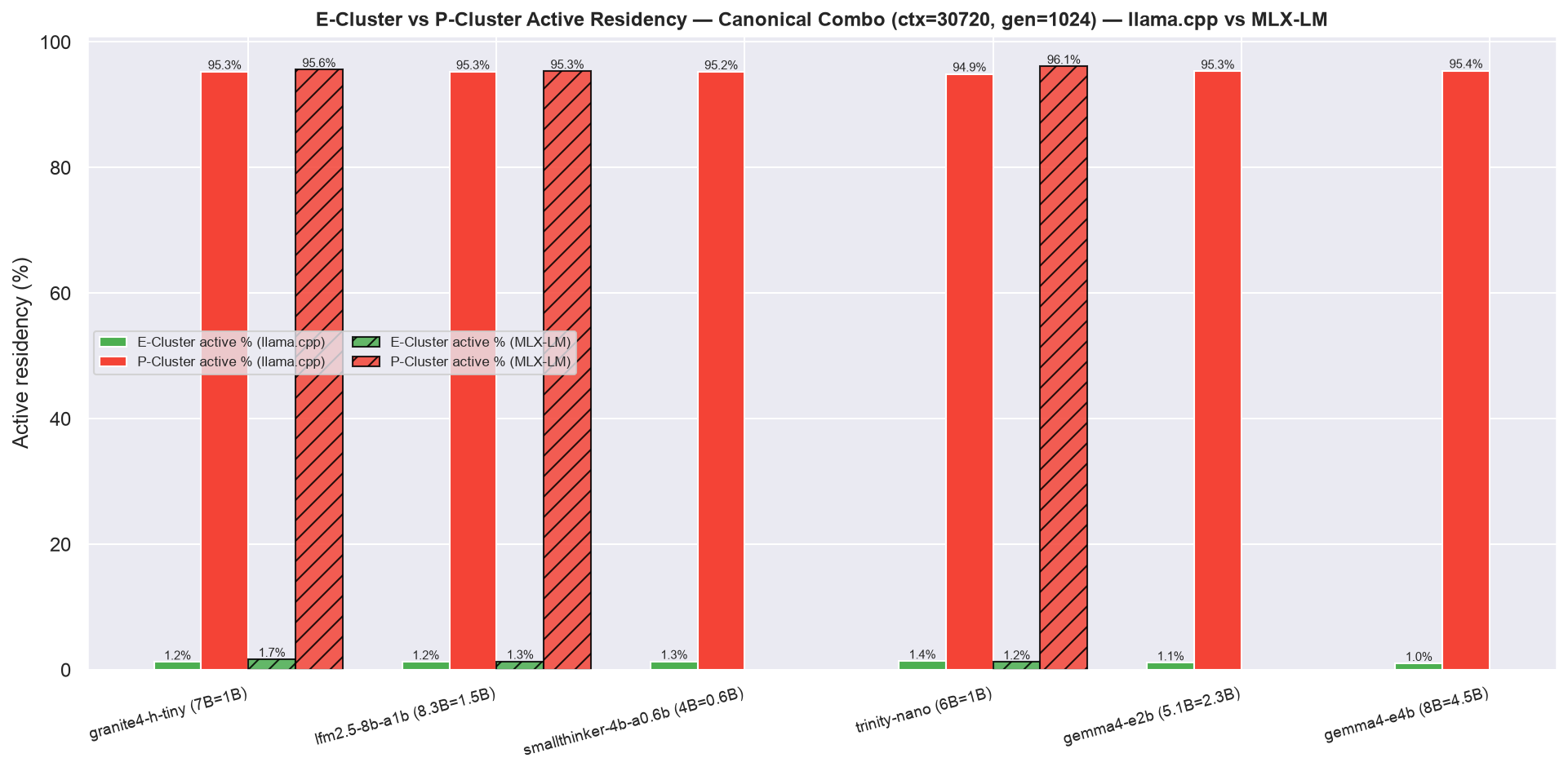
Table 11 and Table 11b give the per-model canonical-cell E-/P-cluster active residency that Figure 10c condenses.
Table 11: CPU cluster active residency at the canonical cell, llama.cpp
| Model | Total Params | Active Params | E-Cluster active (%) | P-Cluster active (%) |
|---|---|---|---|---|
| gemma4-e4b | 8B | 4.5B | 1.01 | 95.43 |
| granite4-h-tiny | 7B | 1B | 1.22 | 95.26 |
| gemma4-e2b | 5.1B | 2.3B | 1.10 | 95.32 |
| lfm2.5-8b-a1b | 8.3B | 1.5B | 1.25 | 95.25 |
| smallthinker-4b-a0.6b | 4B | 0.6B | 1.31 | 95.24 |
| trinity-nano | 6B | 1B | 1.36 | 94.91 |
Table 11b: CPU cluster active residency at the canonical cell, MLX-LM (3 shared models)
| Model | Total Params | Active Params | E-Cluster active (%) | P-Cluster active (%) |
|---|---|---|---|---|
| trinity-nano | 6B | 1B | 1.25 | 96.12 |
| granite4-h-tiny | 7B | 1B | 1.67 | 95.60 |
| lfm2.5-8b-a1b | 8.3B | 1.5B | 1.33 | 95.34 |
At the canonical cell the split is extreme: the 6 efficiency cores sit at ~1.0-1.7 % active residency for every model/backend pair, while the P-cluster holds ~95-96 % - the canonical-cell values condensed by the right-hand column of Figure 10.
Figure 10d and Figure 10e carry the P-Cluster frequency detail at that same canonical combo - the bar summary of average active clock, and the trace over the run.
Figure 10d: Average P-Cluster (performance-core) frequency while active, llama.cpp vs MLX-LM, canonical combo
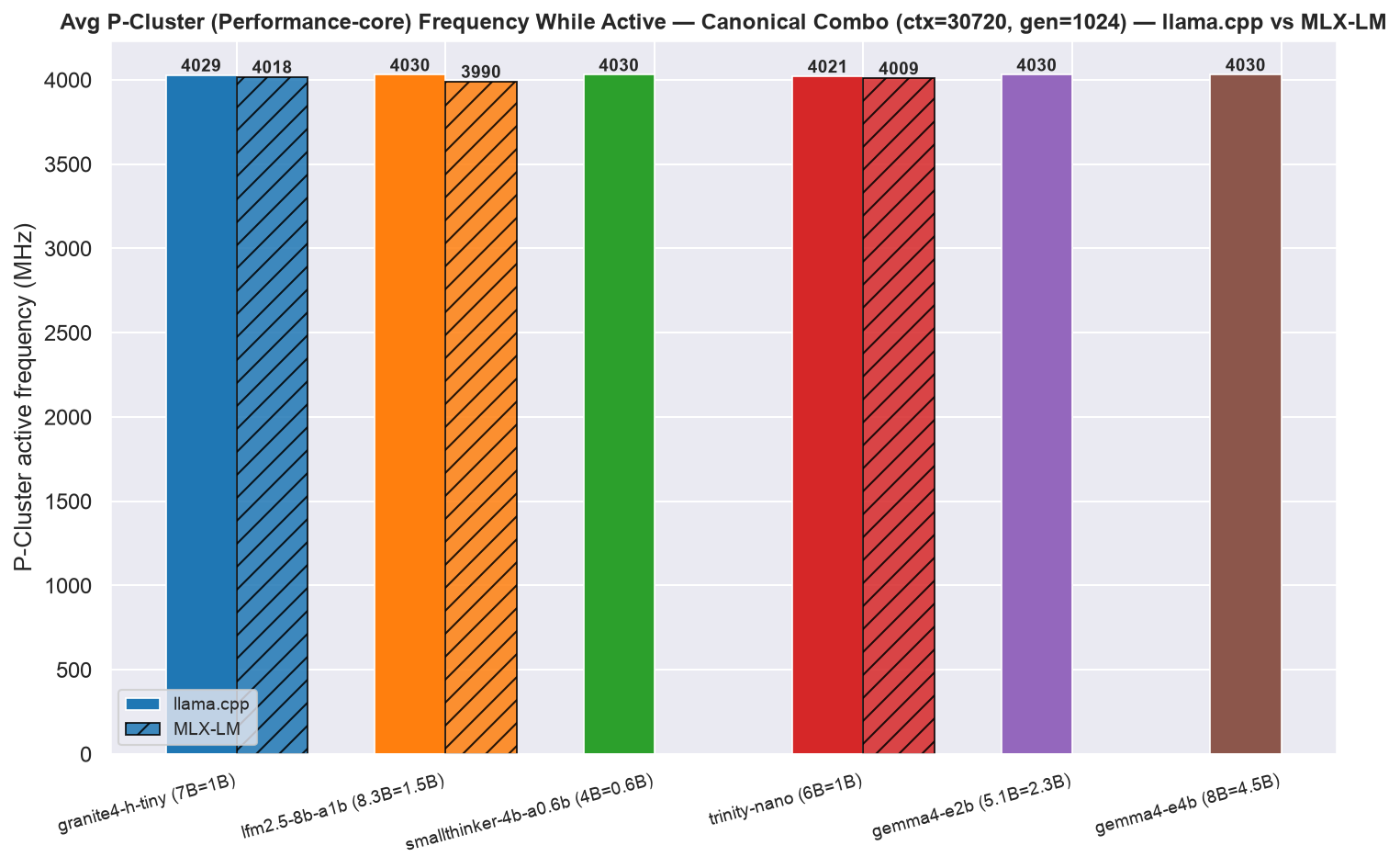
Figure 10e: P-Cluster active frequency over the canonical-combo run, llama.cpp (solid) vs MLX-LM (dashed)
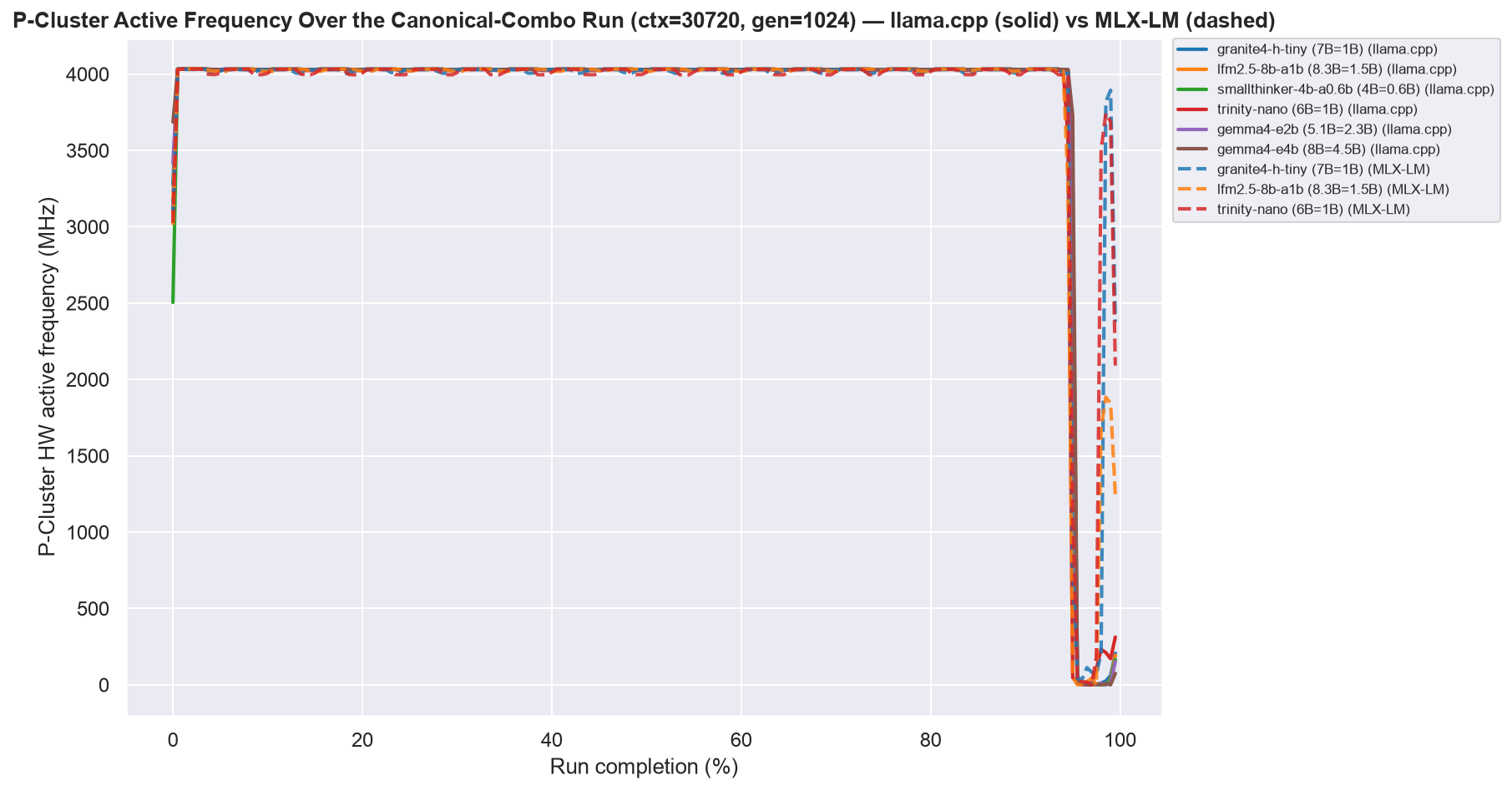
- Every model pins the P-cluster at ~3.99-4.03 GHz for essentially the whole run, under both backends - all nine lines sit on top of each other (llama.cpp 4021-4030 MHz, MLX-LM 3990-4018 MHz). No per-request ramp like the GPU (Figure 9d).
- No Jetson-style
nvpmodelgovernor: the P-cluster never steps down - not between requests, not prefill vs decode, not across models or backends. Only OS DVFS keeps it from a perfectly flat line.
2.7 RSS (Memory) Usage
The third per-process signal sampled alongside powermetrics is RSS (resident set size) - ps -o rss= on the server PID, taken every 50 ms for the whole combo (Appendix I.13). It’s model weights + KV-cache + activations together, not a fixed “model size” number. Figure 11 charts peak RSS across the full sweep; the sweep’s long-context end (the canonical combo’s 30,720-token prompt, where the KV-cache component is largest) is then kept as the exemplar endpoint in Figure 11b. Both backends are charted: llama.cpp all 6 models (solid), MLX-LM the 3 shared models (dashed).
Figure 11: Peak RSS vs prompt length, all models, all 3 generation lengths (gen=256/512/1024), llama.cpp (solid) vs MLX-LM (dashed)
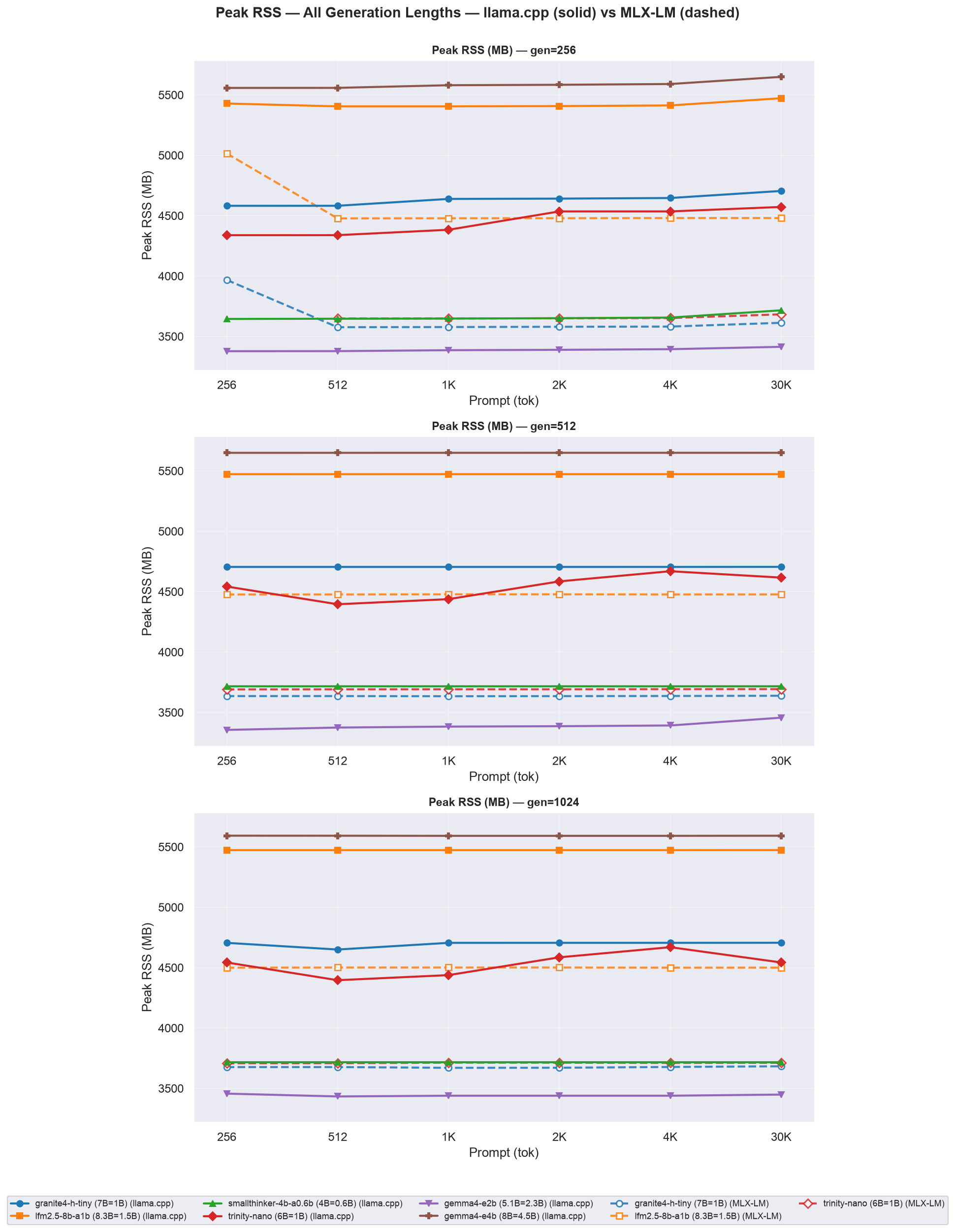
- Peak RSS rises with prompt length then plateaus - llama.cpp reaches its sweep max by ctx≈512-4096 and stays flat to 30,720. A couple of MLX-LM short-ctx peaks (e.g. Granite 3,968 MB at ctx=256) are first-request transients; read the trend from the llama.cpp lines. Largest footprint: Gemma-4-E4B under llama.cpp (5,650 MB), still >10 GB free on the 16 GB pool.
- The llama.cpp-vs-MLX-LM ordering never flips: llama.cpp holds more peak RSS than MLX-LM for all three shared models at every cell - the one metric here with no context-dependent crossover.
Figure 11b: Server process RSS over the canonical-combo run, llama.cpp (solid) vs MLX-LM (dashed) (ctx=30720, gen=1024)
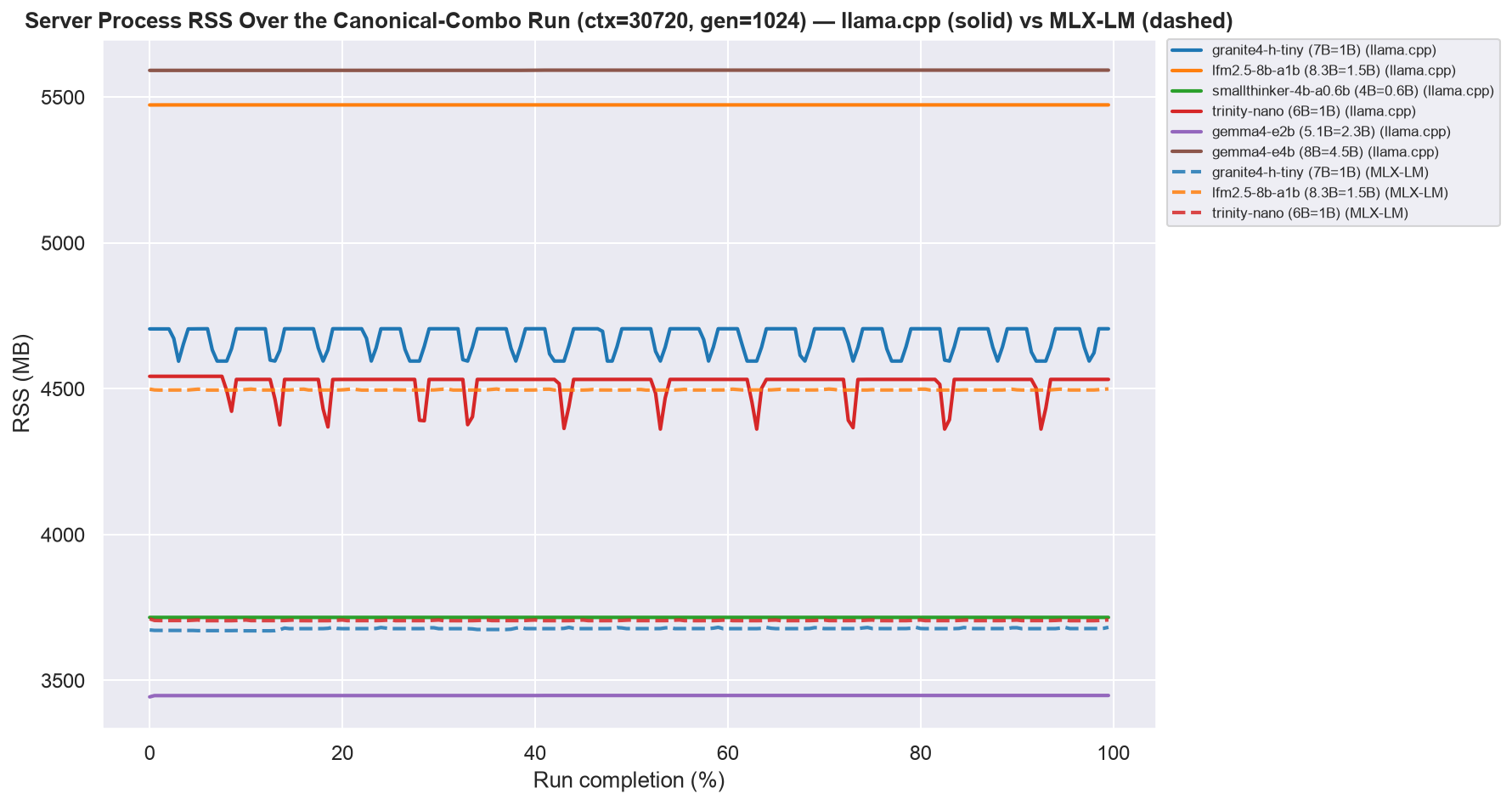
Peak values at the long-context end match the Peak RAM columns of Table 1 (llama.cpp) and Table 2 (MLX-LM) exactly (3.4-5.6 GB llama.cpp, 3.7-4.5 GB MLX-LM). MLX-LM’s peak RSS is lower than llama.cpp’s for all 3 shared models (granite4-h-tiny: 3683 MB vs 4706 MB; lfm2.5-8b-a1b: 4500 MB vs 5473 MB; trinity-nano: 3712 MB vs 4543 MB) - a 17.8-21.7 % reduction, plausibly from MLX’s array framework packing the KV-cache more tightly than GGML’s buffer allocator at this context length.
- Shape, not just peak: under llama.cpp, Granite and Trinity show a sawtooth (RSS drops ~100-180 MB between requests) while LFM2.5, SmallThinker, and both Gemma-4s stay flat - consistent with Granite/Trinity releasing the freed KV buffer between requests (
--no-cache-prompt --cache-ram 0disables reuse for every model alike). - Under MLX-LM the pattern partly inverts: Granite’s dashed line is flat, Trinity’s still dips - behaviour varies by backend and model, not architecture alone.
All six models stay well inside the Mac Mini M4’s 16 GB unified pool even at this longest-context cell, under either backend - the largest footprint (Gemma-4-E4B under llama.cpp, 5.6 GB) leaves more than 10 GB of headroom for the OS and other processes.
Table 12 condenses the sweep to each model’s median across all 18 combos peak RSS, per backend:
Table 12: Median across all 18 combos - peak RSS, per model and backend (llama.cpp vs MLX-LM)
| Model | Total Params | Active Params | Peak RSS (MB) llama.cpp | Peak RSS (MB) MLX-LM |
|---|---|---|---|---|
| gemma4-e4b | 8B | 4.5B | 5592 | - |
| gemma4-e2b | 5.1B | 2.3B | 3393 | - |
| granite4-h-tiny | 7B | 1B | 4704 | 3635 |
| lfm2.5-8b-a1b | 8.3B | 1.5B | 5473 | 4479 |
| smallthinker-4b-a0.6b | 4B | 0.6B | 3716 | - |
| trinity-nano | 6B | 1B | 4539 | 3691 |
The same comparison as Table 6/Table 7, for peak RSS. The llama.cpp-vs-MLX-LM ordering never flips at the median cell - llama.cpp holds more peak RSS for all three shared models.
3. Analysis
3.1 Higher output tok/s != efficient model (tok/J)
The same sweep ranked two different ways: Figure 2 takes each model’s best tok/s, Figure 4 takes its best tok/J. The fastest cell for a model is not always its most efficient one.
The identity behind that makes the two rankings easy to reason about. With output tok/J defined on decode energy only,
tok/J = tok/s ÷ decode_power_W- verified against all 161 reported cells to within 1.3 %. So a model wins on efficiency either by decoding faster at equal decode power, or by decoding at the same speed for less power; the two rankings diverge whenever one model is faster and the other is cooler.
- SmallThinker-4B-A0.6B is the sharpest example. At ctx=256 it is fastest at gen=256 (130.75 tok/s) but least efficient of its three gen lengths there (8.24 tok/J); at gen=1024 (same ctx=256) it is slightly slower (126.42 tok/s) but most efficient (8.82 tok/J) - a longer generation amortizes the fixed prefill energy over more output tokens. Its single best cell anywhere in the sweep is actually ctx=512, gen=1024 (8.97 tok/J, the highest value in the entire dataset).
Table 13: SmallThinker-4B-A0.6B - tok/s vs tok/J crossover at ctx=256 vs ctx=30720
| Gen length | Tok/s @ ctx=256 | Tok/J @ ctx=256 | Tok/s @ ctx=30720 | Tok/J @ ctx=30720 |
|---|---|---|---|---|
| 256 | 130.75 | 8.24 | 55.47 | 3.92 |
| 512 | 129.51 | 8.18 | 55.34 | 3.92 |
| 1024 | 126.42 | 8.82 | 55.04 | 3.88 |
- Unlike the Jetson power-mode case, there is no clock/power tradeoff driving this on Apple Silicon (single operating point) - the driver here is purely generation length amortizing prefill energy, and separately, context length collapsing throughput (see 3.2).
3.2 Context-Length Retention: the short-context leader is not the long-context leader
Figure 12: Output tok/s retained at ctx=30720 vs ctx=256 (gen=1024)
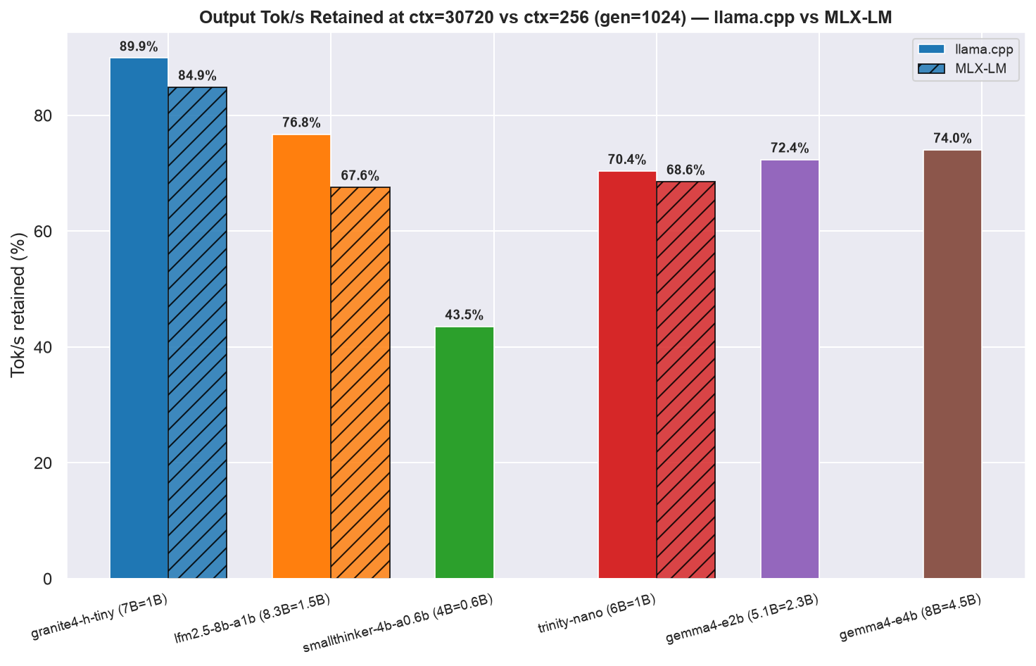
Table 14: Context-length retention, llama.cpp (gen=1024)
| Model | Total Params | Active Params | Tok/s @ ctx=256 | Tok/s @ ctx=30720 | Retained |
|---|---|---|---|---|---|
| granite4-h-tiny | 7B | 1B | 50.6 | 45.5 | 89.9 % |
| lfm2.5-8b-a1b | 8.3B | 1.5B | 83.0 | 63.7 | 76.7 % |
| trinity-nano | 6B | 1B | 86.8 | 61.1 | 70.4 % |
| gemma4-e4b | 8B | 4.5B | 30.4 | 22.5 | 74.0 % |
| gemma4-e2b | 5.1B | 2.3B | 58.1 | 42.0 | 72.4 % |
| smallthinker-4b-a0.6b | 4B | 0.6B | 126.4 | 55.0 | 43.5 % |
Across the sweep the ordering is not stable: SmallThinker-4B-A0.6B wins every short-context cell but is overtaken by LFM2.5-8B-A1B and Trinity-Nano-Preview by the long-context end of the sweep (ctx=30,720) - it retains less than half its ctx=256 throughput by then, the steepest decay of any model tested, while Granite-4.0-H-Tiny (the slowest model at short context) is the most context-stable, retaining 90 % across the whole span. This is the single most important nuance in this benchmark: “fastest model” is not a fixed label - it depends on the context length of the workload.
The retention crossover is visualized in Figure 12 and tabulated in Table 14.
- Table 14 is llama.cpp-only - and under MLX-LM the two 1B-active models actually cross over at long context.
- Retention is nearly the same under both backends (consistent with being a model property): replaying the same
gen=1024cells under MLX-LM givesgranite4-h-tiny84.9 % (69.99 → 59.41 tok/s) andtrinity-nano68.6 % (80.37 → 55.11) - within a few points of their llama.cpp retention above.- What does change between backends is the short-context baseline:
granite4-h-tinyis +38 % faster at ctx=256 under MLX-LM (70.0 vs 50.6 tok/s), whiletrinity-nanois -7 % slower (80.4 vs 86.8).- Flat retention × a healthy baseline inverts the ordering under MLX-LM between ctx=4096 and ctx=30720:
trinity-nanoleads by 7-15 % through ctx=4096, thengranite4-h-tinyleads by +7.8 % (59.4 vs 55.1 tok/s) at the long-context end of the sweep - the dashed lines crossing in Figure 1.- Under llama.cpp no crossover occurs inside the sweep: Granite’s baseline (50.6 vs 86.8) is too far behind for its flatter slope to close the gap within 30k tokens.
- Bottom line: the flat curve travels with the model (visible under both backends); the baseline travels with the backend - llama.cpp’s Metal path is much harder on the Mamba-2 hybrid than MLX-LM’s.
3.3 Best Total tok/J per Model - Ranked by Peak Throughput (llama.cpp)
Table 15 reports the llama.cpp maxima, and Table 16 reports the MLX-LM maxima.
Table 15: Best total tok/J per model, searched across all 18 llama.cpp combos
| Model | Total Params | Active Params | Best total tok/J | At ctx / gen |
|---|---|---|---|---|
| smallthinker-4b-a0.6b | 4B | 0.6B | 51.48 | 4096 / 256 |
| trinity-nano | 6B | 1B | 46.90 | 30720 / 256 |
| lfm2.5-8b-a1b | 8.3B | 1.5B | 35.16 | 30720 / 256 |
| gemma4-e2b | 5.1B | 2.3B | 25.02 | 30720 / 256 |
| granite4-h-tiny | 7B | 1B | 29.42 | 30720 / 256 |
| gemma4-e4b | 8B | 4.5B | 14.56 | 30720 / 256 |
- Total tok/J = (
ISL+OSL) / (prefill_J+decode_J) - the phase-summed request energy per Appendix I.5/I.6, not the whole-requestavg_power_W × RLestimate in Appendix I.4.- Five of the six models peak at the longest-prompt / shortest-generation cell (ctx=30720, gen=256) - expected from the formula, since the (ISL+OSL) numerator grows with the prompt while the short decode keeps the denominator low.
- SmallThinker is the exception: it peaks at ctx=4096, gen=256, the model whose prefill energy grows fastest with context (see Table 13).
Table 16: Best total tok/J per model, MLX-LM (3 models)
| Model | Total Params | Active Params | Best total tok/J | At ctx / gen |
|---|---|---|---|---|
| trinity-nano | 6B | 1B | 46.98 | 30720 / 256 |
| lfm2.5-8b-a1b | 8.3B | 1.5B | 37.71 | 30720 / 256 |
| granite4-h-tiny | 7B | 1B | 35.45 | 30720 / 256 |
3.4 Latency Characteristics
TTFT scales near-linearly with prompt length. Across the sweep it rises from well under a second at ctx=256 to 34.1-112.6 s depending on model at the long-context end (ctx=30720) - by far the dominant term in end-to-end request latency there (see Figure 5).
Inter-token latency (ITL) p50, the median per-token decode cost, compresses across the sweep: the models separate widely at short context but converge as context grows.
- Gemma-4-E4B has by far the highest ITL at every cell tested (44.4 ms/tok, i.e. ~22.5 tok/s decode, at the long-context end) - consistent with it being the largest model and the slowest throughout.
- SmallThinker-4B-A0.6B, Trinity-Nano-Preview, and LFM2.5-8B-A1B cluster tightly (15.7-18.2 ms/tok) at the long-context end despite having very different ITL at short context - context length compresses the gap between the faster models more than it widens it.
Peak RAM (RSS) scales with context length as the KV-cache grows, on top of a per-model baseline footprint. At ctx=256, footprints range from 3.4 GB (Gemma-4-E2B) to 5.6 GB (Gemma-4-E4B) - all comfortably inside the Mac Mini M4’s 16 GB unified pool even before accounting for the OS and other processes. Full peak-RAM heatmaps are in Appendix I.2 (i2g_peak_ram.png).
3.5 Prefill vs Decode Energy Split
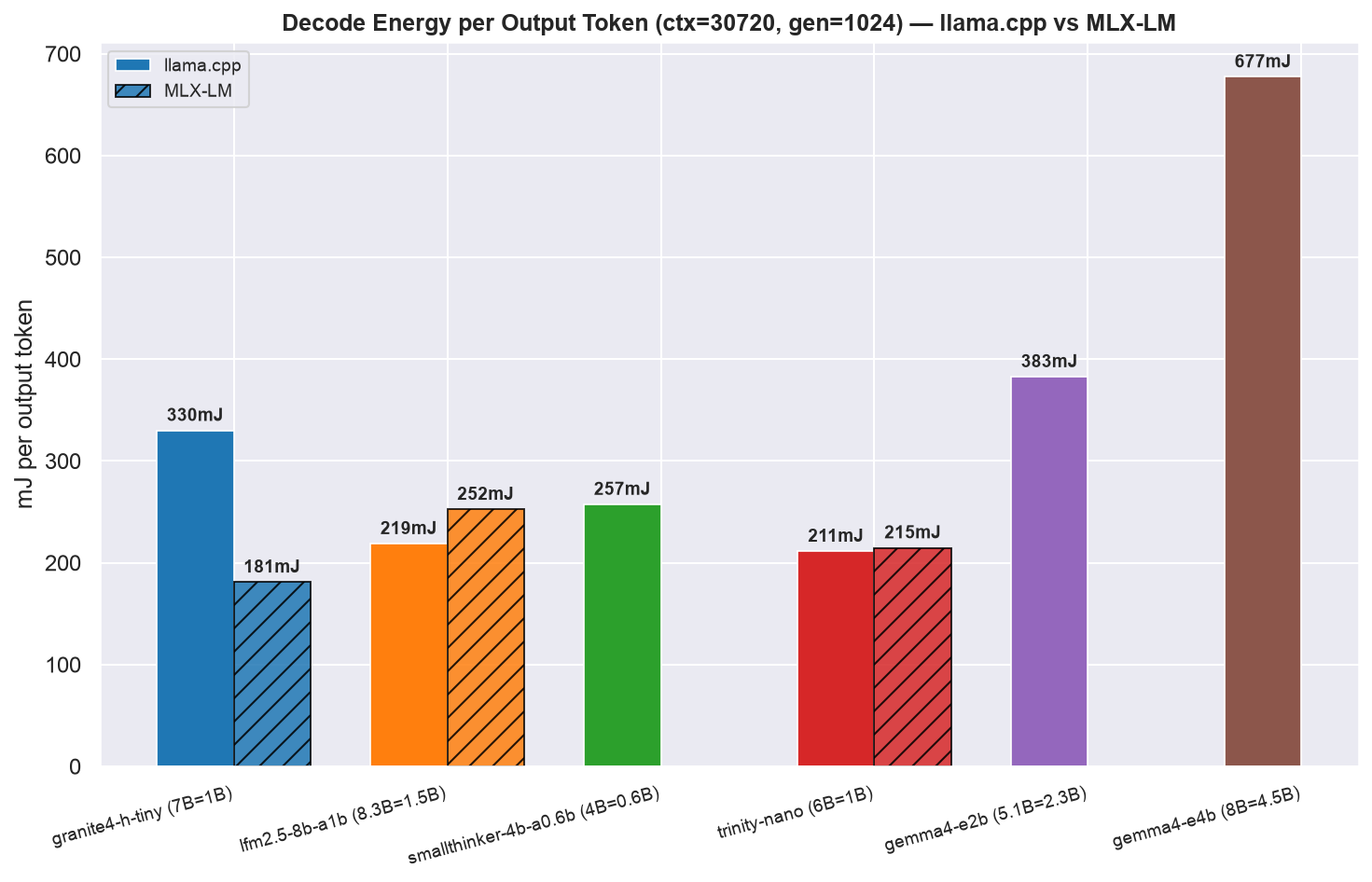
Figure 13 shows how request energy divides between prefill and decode, while Figure 14 normalizes decode energy per output token at the canonical cell.
Figure 13: Request energy split - prefill % vs decode % (median across the sweep; the run’s first cell is excluded as warm-up, §1.4)
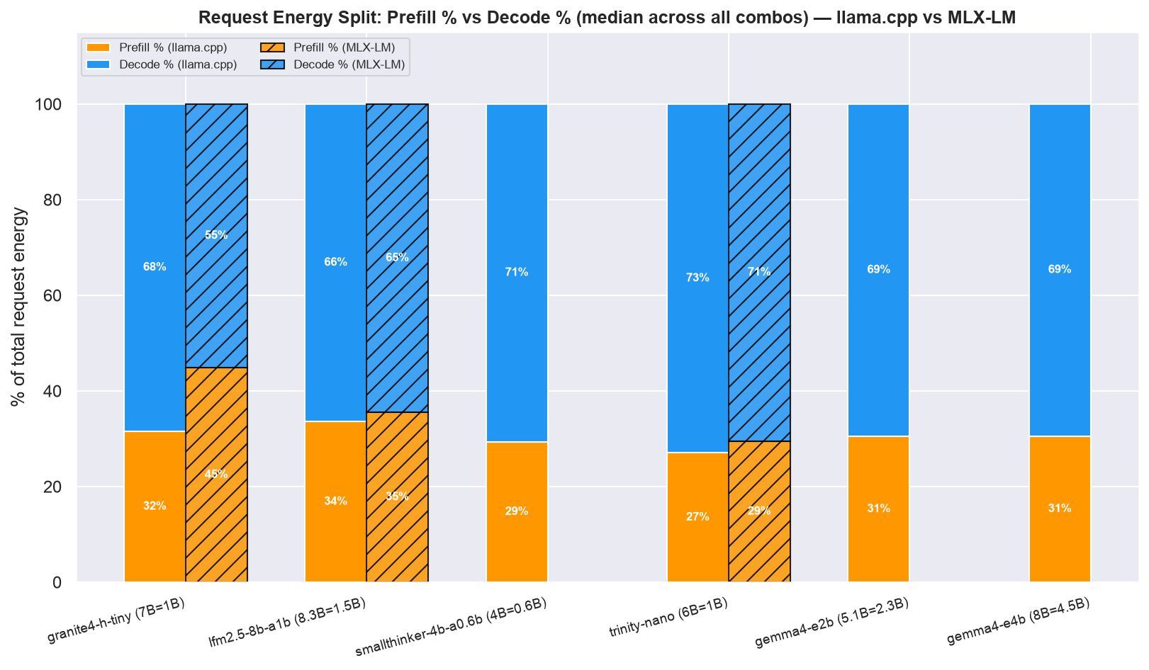
Figure 14: Decode energy per output token (mJ), canonical cell
- At short-to-medium context, decode energy dominates the request (many output tokens, one prefill). As context grows toward the 30,720-token canonical cell, prefill energy takes over the request-energy budget for every model - directly visible in Figure 3 (total tok/J rising with context while decode tok/J in Figure 3 falls).
-
SmallThinker-4B-A0.6B’s decode-phase energy per output token is the lowest of any model at short context, consistent with its top tok/J numbers in Table 13.
- The same prefill/decode split explains the backend efficiency gap.
- Prefill tok/J is near-parity for the shared models - prefill is compute-bound and both backends saturate the GPU alike.
- Output tok/J carries the divergence (the decode phase) and flips with context: at the long-context end Granite swings decisively toward MLX-LM (which streams its Mamba/MoE weights far faster), while LFM2.5 and Trinity stay at or above parity.
- So Granite’s MLX-LM win is a decode-phase effect, not a prefill one.
- The efficiency winner for LFM2.5/Trinity flips with context length rather than being a blanket llama.cpp win (see 4.2); per-cell
LC ÷ MXvalues are in Table 17.
4. Backend Comparison: llama.cpp vs MLX-LM
Both backends ran identical Q4_K_M / 4-bit-MLX quantizations at single-user concurrency on the same Mac Mini M4. Three of the six models have data under both backends - see caveats for why the other three are llama.cpp-only.
4.1 Throughput and Efficiency Head-to-Head
Table 17 is the head-to-head at the long-context end of the sweep (ctx=30720, gen=1024 - the canonical cell), used here as the exemplar endpoint; §4.2 generalizes each pattern across the full sweep.
Table 17: llama.cpp vs MLX-LM at the long-context end of the sweep (ctx=30720, gen=1024 - the canonical cell)
| Model | Total Params | Active Params | llama.cpp tok/s |
MLX-LM tok/s |
LC ÷ MX | llama.cpp tok/J |
MLX-LM tok/J |
LC ÷ MX tok/J |
|---|---|---|---|---|---|---|---|---|
| Granite-4.0-H-Tiny | 7B | 1B | 45.45 | 59.41 | 0.77× | 3.0197 | 5.4884 | 0.55× |
| LFM2.5-8B-A1B | 8.3B | 1.5B | 63.73 | 54.99 | 1.16× | 4.5605 | 3.8666 | 1.18× |
| Trinity-Nano-Preview | 6B | 1B | 61.08 | 55.11 | 1.11× | 4.6884 | 4.6413 | 1.01× |
4.2 Key Observations
1. There is no universal winner between backends on Apple Silicon.
Unlike the Jetson CUDA case, where llama.cpp beat Ollama for almost every model, here the result is split: MLX-LM wins decisively for Granite-4.0-H-Tiny, while llama.cpp wins narrowly for LFM2.5-8B-A1B and Trinity-Nano-Preview. This suggests the two frameworks’ kernel optimisation priorities diverge by architecture (hybrid Mamba/attention vs. hybrid SSM/attention vs. standard MoE routing) rather than one framework being categorically faster on this hardware.
2. MLX-LM draws less power for the same work - consistently across the sweep.
Across all three shared models, MLX-LM’s median total power across the sweep (10.4-12.3 W) is consistently lower than llama.cpp’s (12.6-14.4 W) - see Figure 8. This is plausibly server/framework overhead rather than raw compute efficiency: the tok/J gap is wider than the power gap alone would predict (Granite reaches 1.8× at the long-context end, from 10.84 W vs 15.07 W decode power, because MLX-LM is also ~1.3× faster on throughput there).
3. Best-of-both-worlds recommendation.
The resulting workload-specific choices are summarized in Table 18.
Table 18: Recommended backend and model by use case
| Use case | Backend | Model |
|---|---|---|
| Max long-context throughput | llama.cpp | LFM2.5-8B-A1B |
| Max short-context throughput / efficiency | llama.cpp | SmallThinker-4B-A0.6B (no MLX weights published) |
| Granite family on Apple Silicon | MLX-LM | Granite-4.0-H-Tiny |
| Lowest average power for a given model | MLX-LM | any of the 3 shared models |
4.3 Data-Quality Caveat: MLX-LM Generation-Length Undershoot
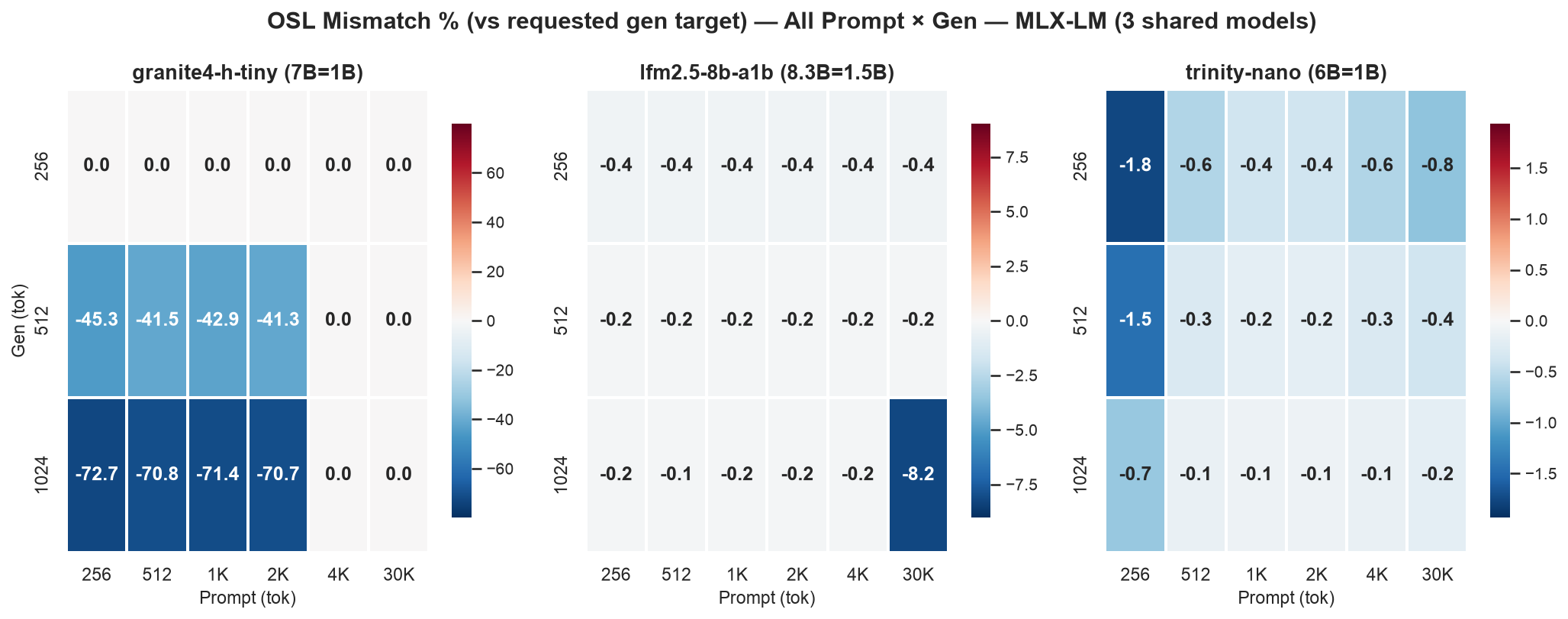
--ignore-eos on llama.cpp forces every request to produce exactly the target gen token count; MLX-LM’s server has no equivalent flag, so it stops as soon as the model emits an EOS token. For most models this causes only a small (<5 %) OSL undershoot. Granite-4.0-H-Tiny under MLX-LM is a severe outlier: at gen=512 and gen=1024 targets, actual output length falls 40-72 % short of target (e.g. 292.5 tokens actually generated against a 1024-token target, p50). Under llama.cpp, the same model’s OSL matches its target almost exactly (<3 % deviation) at every combo.
This means Granite-4.0-H-Tiny’s MLX-LM tok/s and tok/J numbers at longer gen targets are computed over a shorter-than-intended generation window - a backend-specific early-stopping behaviour, not a hardware or power effect. Treat the MLX-LM Granite comparison in Table 17 as directionally correct but not perfectly apples-to-apples with the llama.cpp row for that model. Full per-cell OSL mismatch appears in Figure I.2c for llama.cpp and Figure I.2d for MLX-LM.
5. Conclusion
What These Numbers Mean for Local Inference on Apple Silicon
Small MoE/hybrid-MoE inference on a $599 Mac Mini M4 16GB is practical well past the token counts most local-LLM benchmarks test. Across the full ctx=256 → 30,720 sweep:
- Every model fits comfortably inside 16 GB unified memory at every cell tested, with 3-6 GB of headroom to spare
- No model throttled at any point across either backend’s full sweep - the M4’s cooling handles sustained MoE inference without a power-mode governor to fall back on
- Throughput degrades gracefully: the worst-retaining model still keeps 43.5 % of its short-context speed by the long-context end, and the best keeps 90 % - so no model falls off a cliff inside the sweep
- At the long-context end (ctx=30,720 - the canonical cell), LFM2.5-8B-A1B sustains 63.7 tok/s - real-time-adjacent generation even with a full long document loaded
- SmallThinker-4B-A0.6B is the fastest model in the suite at any context under ~4k tokens (130.75 tok/s at ctx=256), and the single most tok/J-efficient cell in the entire sweep (8.97 at ctx=512, gen=1024)
The Two Practical Takeaways
- Match the model to your context length, not just its published benchmark numbers. SmallThinker-4B-A0.6B’s short-context throughput crown means little if your workload routinely sends 20k+ token prompts - by the long-context end it is the slowest model in this suite, having lost more than half its speed. Check retention (Table 14), not just peak tok/s.
- Match the backend to the model, not a blanket “llama.cpp is faster” assumption. That held on Jetson/CUDA; it does not hold cleanly here. Granite-4.0-H-Tiny specifically favors MLX-LM; benchmark your own model/backend pair before committing to one framework project-wide.
What Is Not Yet Benchmarked
- Multi-user concurrency: all results are single-user (
--parallel 1/--decode-concurrency 1). Real-world serving will see different throughput/latency profiles at concurrency > 1. - Neural Engine (ANE) offload: neither backend under test routes any compute through the M4’s 16-core ANE; an ANE-aware runtime could shift the power/throughput picture materially.
- SmallThinker under MLX-LM: no 4-bit MLX conversion is currently published for this model; if one becomes available, it is the most interesting backend comparison left to run given its short-context dominance under llama.cpp.
- Gemma-4-E2B/E4B under MLX-LM: blocked on
mlx_vlm.serversupport for the native VLM weight structure - see backend caveats.
Appendix A: Prefill vs Decode Power Split - All Generation Lengths
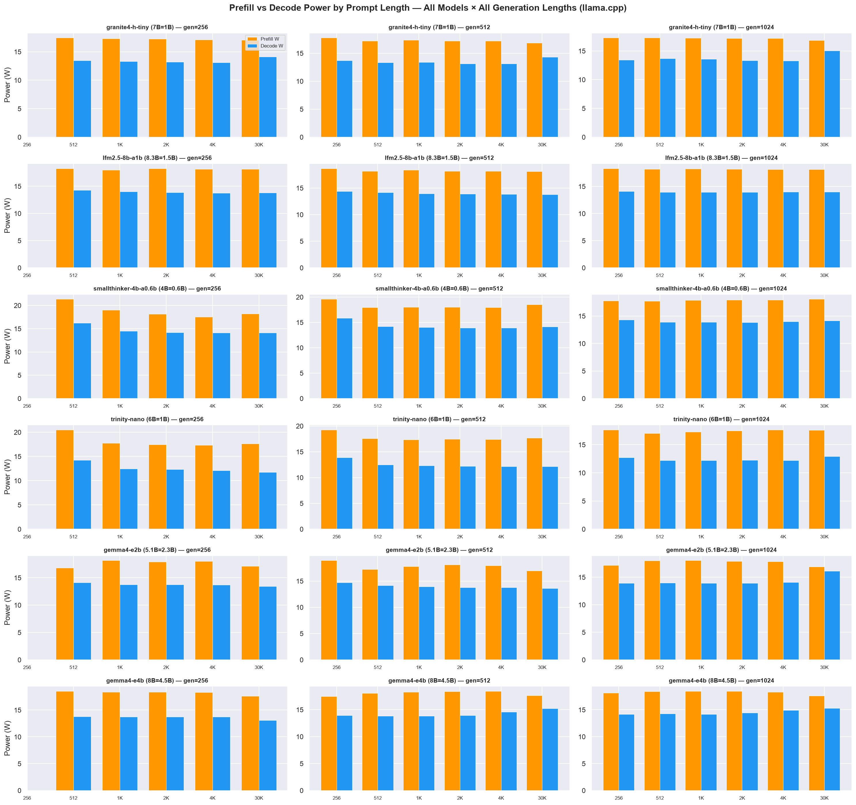
The all-generation latency and power line charts are the §2-ordered Figure 5 and Figure 7, so this appendix does not re-cite them; it keeps only the power view those lines don’t show - the phase-resolved prefill-vs-decode power split by prompt length in Figure A.1. It is a 6 model × 3 gen panel grid, so the full sweep is shown rather than a single gen slice.
Figure A.1 - Prefill vs decode power by prompt length, all 6 models × all 3 generation lengths (llama.cpp, complete 6-model dataset)
Appendix B: Request-Latency Percentile Detail (Canonical Cell)
The full-sweep line charts for the latency and throughput signals are in section 2 - latency (TTFT / ITL / RL) in Figure 5, output/prefill throughput in Figure 1 - so this appendix does not repeat them as per-cell heatmaps. It keeps only the one view those grids don’t already show: the canonical-cell percentile spread of request latency. (The only per-cell heatmap left in the report is the OSL-mismatch grid in Appendix I.2.)
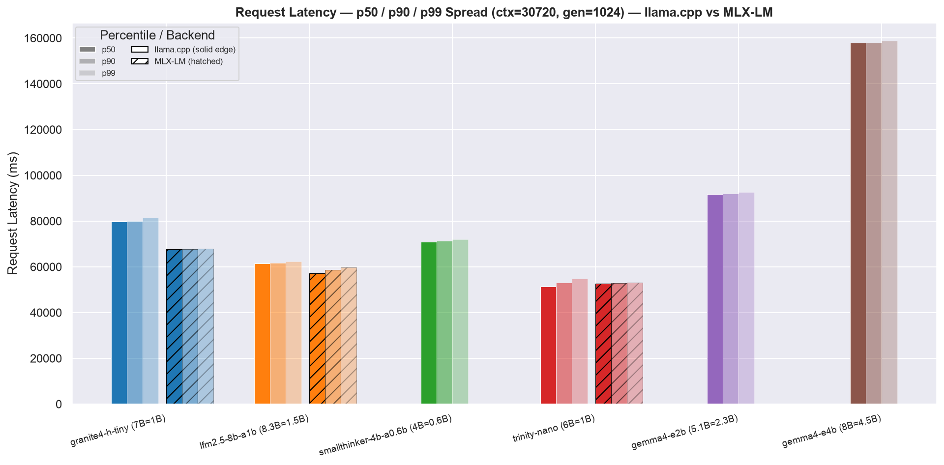
B.1 Request latency percentile spread (canonical cell)
Figure B.1: Request latency p50/p90/p99 spread at the canonical cell, llama.cpp (solid edge) vs MLX-LM (hatched)
Appendix I.2: Extended Dashboard Charts
Supplementary charts covering the full 18-combo × 6-model dataset from angles not already shown as sweep line charts in section 2: a data-quality signal (OSL mismatch) plus two non-line encodings. The compact all-combo line grids for tok/s, tok/J, latency and power live in §2 - the old per-cell heatmap re-encodings of those same sweeps have been retired.
- Tok/J by generation length: Figure I.2a
- Peak RAM: Figure I.2b
- OSL mismatch: Figure I.2c and Figure I.2d
Figure I.2a: Tok/J grouped bars by generation length (llama.cpp, complete 6-model dataset)
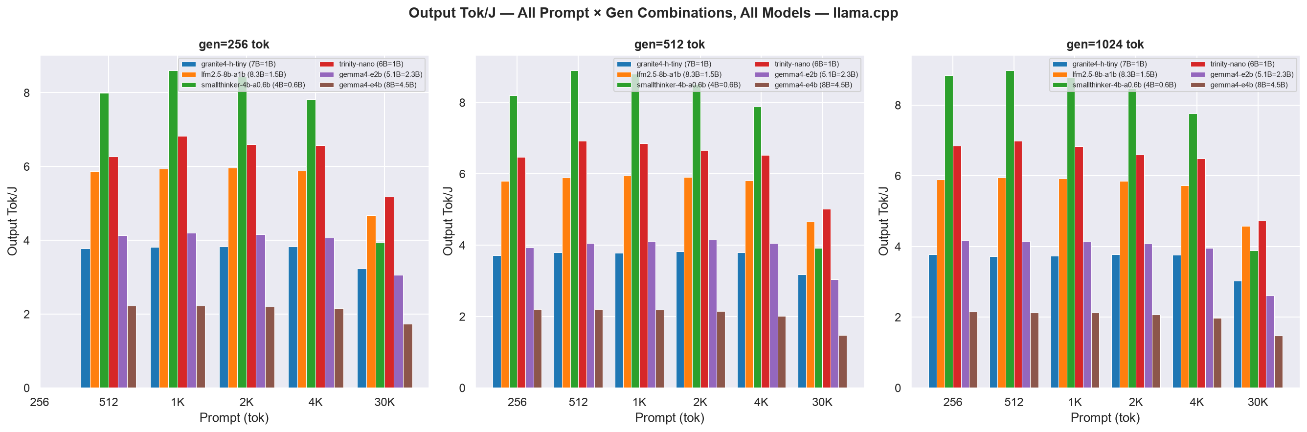
Figure I.2b: Peak RAM (RSS) by model, llama.cpp vs MLX-LM (max across all combos each backend ran)
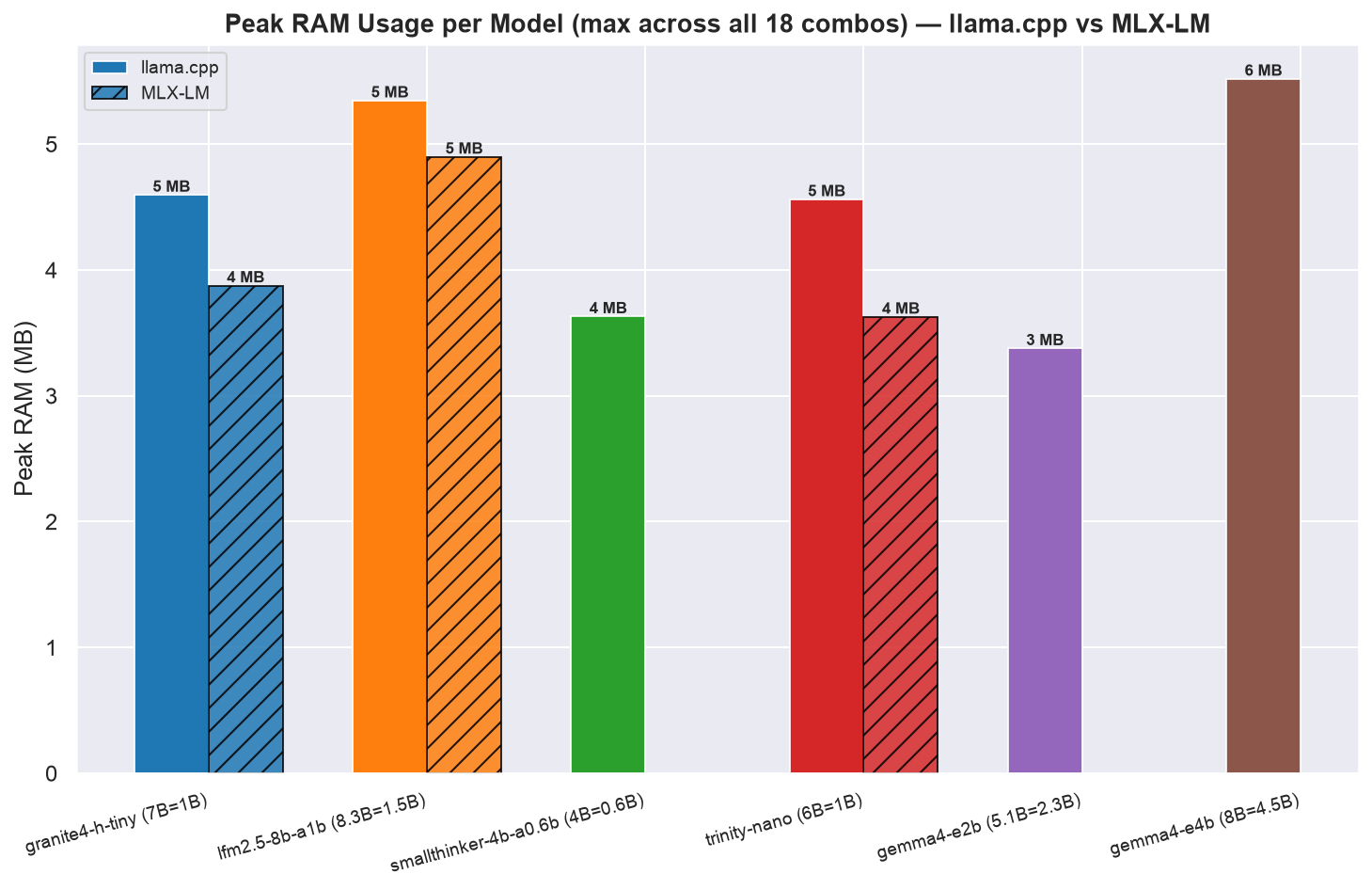
Figure I.2c: OSL mismatch heatmap - actual vs target output tokens, all models × all combos, llama.cpp
Figure I.2c shows that every llama.cpp cell stays within a few percent of target thanks to --ignore-eos.
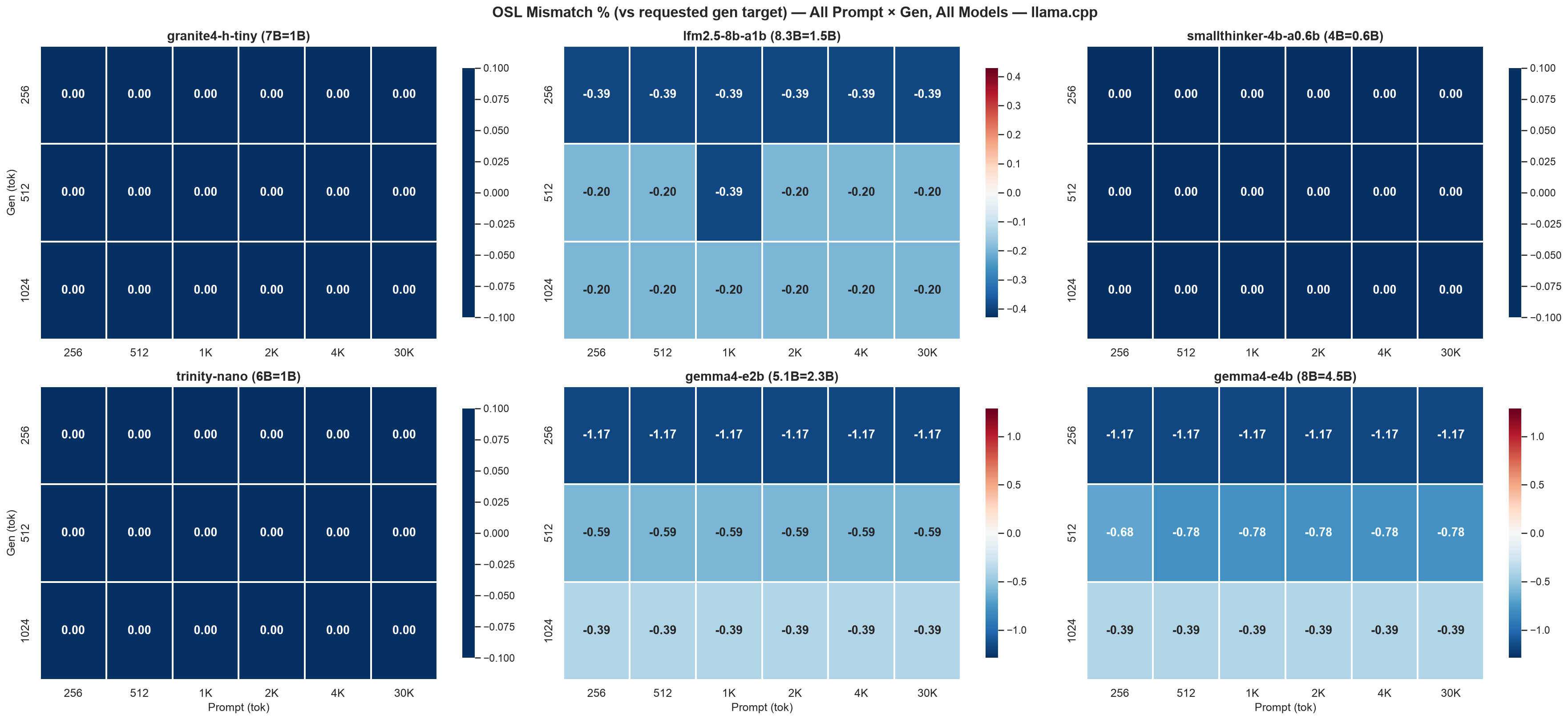
Figure I.2d: OSL mismatch heatmap, MLX-LM (3 shared models)
Figure I.2d confirms the section 4.3 MLX-LM Granite undershoot directly: -70.7 to -72.7 % at gen=1024 and -41.3 to -45.3 % at gen=512, vs single-digit-percent deviation for lfm2.5-8b-a1b and trinity-nano at every combo.
Appendix I: All Metrics, Formulas, and Calculation Methods
This appendix documents every metric reported in this benchmark, its formula, its source, and any caveats.
I.1 Raw inputs from aiperf and powermetrics
Table I.1 defines the raw inputs used by the formulas in this appendix.
Table I.1: Raw metric inputs, sources, and definitions
| Symbol | Source | Definition |
|---|---|---|
ISL |
aiperf JSON input_sequence_length.p50 |
Actual input tokens processed per request (may differ from target due to tokenizer rounding) |
OSL |
aiperf JSON output_sequence_length.p50 |
Actual output tokens generated per request - see 4.3 for the MLX-LM undershoot caveat |
TTFT |
aiperf JSON time_to_first_token.p50 (ms) |
Median time from request sent to first output token received; proxy for prefill duration |
ITL |
aiperf JSON inter_token_latency.p50 (ms) |
Median time between consecutive output tokens; per-token decode cost |
RL |
aiperf JSON request_latency.p50 (ms) |
Median total wall time per request: TTFT + all inter-token intervals |
tok_s |
aiperf JSON output_token_throughput_per_user.p50 |
Output tokens per second, single-user |
prefill_tput |
aiperf JSON prefill_throughput_per_user.p50 |
Input tokens processed per second during prefill phase |
p50_decode_s |
computed | Median decode duration in seconds, from per-request timestamps in profile_export.jsonl, or (RL_p50 - TTFT_p50) / 1000 as fallback |
t0, t1 |
aiperf JSON start_time, end_time (ISO 8601) |
Wall-clock start and end of the full 20-request profiling run |
mW_i |
powermetrics Combined Power (CPU + GPU + ANE) field (mW) |
Instantaneous combined-rail power at sample i |
Two distinct throughput metrics - do not conflate them. Output tok/s is the median rate of generated tokens (aiperf
output_token_throughput_per_user.p50-OSLover the decode window); this is the headline “tok/s” used throughout sections 2-4. Prefill tok/s is the rate of input tokens processed during the prefill phase (aiperfprefill_throughput_per_user.p50). Same units, different phase and different measurement window - the two move with context length in opposite directions and are never interchangeable.
I.2 Power
total_power_W = avg_power_W = median(mW_i for all powermetrics samples in the combo window) / 1000
total_power_W(also writtenavg_power_W) is the whole-combo total power - the “Total Power” line in Figure 7 / Figure 8. It is the median over everypowermetricssample in the combo window (prefill + decode + inter-request idle) - the same estimator as the phase powers, so the only difference between the three columns of Figure 7 is the window, not the statistic. It is still not the sum of the phase powers:prefill_power_Wanddecode_power_W(I.5) are medians over their own windows only, while the combo window also contains inter-request idle, sototal_power_W ≠ prefill_power_W + decode_power_W.Combined Power (CPU + GPU + ANE)is macOS’s own accounting of the three on-package power domains that matter for inference; it does not include board-level overhead (storage, USB, display) the way Jetson’sVDD_INdiffers fromVDD_CPU_GPU_CV.powermetricsinterval: requested 50 ms (-i 50), ≈56.4 ms actually achieved (measured mean over the sweep).- Timestamps are whole-second. Each
powermetricsblock header reads e.g.Sampled system activity (Sat Jul 4 03:46:05 2026 +0530), so a naive read collapses ~17-18 consecutive samples onto one timestamp. The block’s own(56.75ms elapsed)field is the real clock: summing it reproduces the run’s wall duration to under a second, and choosing the one sub-second phase that keeps every reconstructed time inside its logged second pins the timeline to within ~±10 ms over a 1000 s run (99.6-100 % of samples round-trip). Phase classification uses these rebuilt times; without the rebuild, short prefill windows silently absorb whole seconds of decode power.
I.3 Output tok/J (main efficiency metric)
output_tok_J = OSL / (decode_power_W * p50_decode_s)
Higher is better. Output tokens generated per joule of decode-phase energy only - the primary metric of this benchmark, and the one used throughout section 2-4.
I.4 Whole-request energy (average-power cross-check)
request_J_avg = avg_power_W * (RL / 1000)
Energy consumed by one average request from first byte sent to last token received, estimated from the combo-wide average power. This is a cross-check only - the tables and charts use the phase-summed total_J from I.5 (prefill_J + decode_J), which separates the high-power prefill spike from the steadier decode rail instead of averaging them into one number.
I.5 Prefill and decode energy
prefill_J  = prefill_power_W * (TTFT / 1000)
decode_J   = decode_power_W  * p50_decode_s
total_J    = prefill_J + decode_J

prefill_%  = prefill_J / total_J * 100
Prefill/decode windows come from profile_export.jsonl per-request timestamps; the phase boundary is the first output token, at request_start_ns + TTFT (using each request’s time_to_first_token), not request_ack_ns. p50_decode_s is the median over requests of request_end_ns − (request_start_ns + TTFT). prefill_power_W / decode_power_W are the medians of the powermetrics samples falling inside those windows, classified using sample times rebuilt to ~56 ms resolution from each block’s elapsed field - the header timestamp alone is only whole-second, which would mis-bucket short prefill windows (see I.2). Falls back to a TTFT/RL timeline reconstruction if the file is absent for a combo (see compute_phase_power in generate_combined_charts.py).
I.6 Phase tok/J metrics
prefill_tok_J = ISL / prefill_J
decode_tok_J  = OSL / decode_J        (== output_tok_J above)
total_tok_J   = (ISL + OSL) / total_J
prefill_tok_J: input tokens processed per joule of prefill energy.decode_tok_J: output tokens generated per joule of decode energy - identical metric to I.3.total_tok_J: all tokens (in + out) per joule of total request energy.
I.7 mJ per output token
mJ_per_output_tok = (decode_J / OSL) * 1000
                  = 1000 / decode_tok_J
Millijoules per generated output token.
I.8 Prefill tok/s (prefill throughput)
prefill_tput (tok/s) = aiperf JSON prefill_throughput_per_user.p50
Input (prompt) tokens processed per second during the prefill phase - distinct from output tok/s, which counts generated tokens over the decode window (see the two-metric note in I.1). Directly from aiperf. Scales with prompt length (longer prompts hit peak GPU utilisation).
I.9 Context-length retention (Table 14 / Figure 12)
retention_% = tok_s(ctx=30720, gen=1024) / tok_s(ctx=256, gen=1024) * 100
Computed per model, llama.cpp only (MLX-LM has 30720-context data for all 3 shared models too, but the headline retention comparison in 3.2 uses the complete 6-model llama.cpp set).
I.10 Best total tok/J per model
best_total_tok_J(model) = max(total_tok_J(gen, ctx))
                          over all gen in {256, 512, 1024}
                          and all ctx in {256, 512, 1024, 2048, 4096, 30720}
The single highest total tok/J value observed for that model across the sweep - up to 18 combinations, but since total_tok_J is power-derived the run’s first cell is excluded as warm-up (§1.4).
I.11 TTFT, ITL, RL percentiles
All percentile variants come directly from aiperf JSON without further computation:
TTFT       = time_to_first_token.p50   (canonical; p50 used everywhere)
TTFT_p90   = time_to_first_token.p90
TTFT_p99   = time_to_first_token.p99
ITL        = inter_token_latency.p50    (canonical; p50 used everywhere)
ITL_p99    = inter_token_latency.p99
RL         = request_latency.p50        (canonical; p50 used everywhere)
RL_p99     = request_latency.p99
I.12 OSL mismatch
OSL_mismatch_% = (OSL_actual - OSL_target) / OSL_target * 100
Reported per combo in report.md. Near-zero for every llama.cpp cell (--ignore-eos forces the target length); can be strongly negative for MLX-LM, especially Granite-4.0-H-Tiny at longer gen targets - see 4.3.
I.13 Peak RAM (RSS)
peak_ram_MB = max(rss_sample for all 50ms samples in the combo window)
Sampled via ps -o rss= on the server process PID. Captures model weights + KV-cache + activations at that specific prompt/gen length - grows with context, not a fixed “model size” figure.
I.14 GPU / CPU utilization (Figure 9-Figure 10)
These two fields come straight from powermetrics’ own GPU-usage / processor-usage section and are used as-is - no reconstruction, unlike the power samples (I.2):
GPU active residency (%)       = mean(GPU HW active residency % over the combo's samples)
GPU avg active frequency (MHz) = mean(GPU HW active frequency MHz over samples where it is > 0)
Both are additionally computed per phase: the same formulas restricted to the prefill window (request_start_ns→first token) and the decode window (first token→request_end_ns), which is what §2.5’s Figures 9-9d plot.
GPU HW active frequency(MHz) - the GPU hardware clock during a sample.powermetricslogs it once per ~56 ms sample, and a value of 0 MHz means the GPU was fully idle in that sample (no work dispatched). Tables 10/10b quote the mean over active samples only (freq > 0), and Figure 9b plots the full distribution of those samples (models pooled; same gen-row × phase-column layout as Figure 9c) - the clock is bimodal (an initial-boost ~1578 MHz state and a thermal-steady ~1470 MHz state, both chosen by Apple’s on-die power controller - this benchmark pins nothing), so a lone mean is a duty-cycle blend of the two and moves with run length, while the violin shows both states directly; Figure 9d shows the within-run shape. Either way the clock does not ramp during prefill: the long sustained prefill sits below the shorter decode that follows it - by 15 MHz (LFM2.5) up to 83 MHz (gemma4-e4b) at ctx=30720, and the gap widens with context (Figure 9b/9d, Tables 10/10b). The whole-run “climb to ~1570 MHz” is the prefill→decode transition, not the prefill itself. Read it as a measured property of this workload on this chip: the likely driver is the governor trading clock against prefill’s higher sustained power draw (17-18 W vs decode’s 12-15 W, Figure 7), but this data cannot pin the mechanism down.GPU HW active residency/GPU idle residency(%) -powermetricsreports this pair for every sample and the two sum to 100 % (active + idle = 100exactly, verified over all samples). Active residency is the share of the sample window the GPU spent executing; idle residency is its complement. The charts plot active residency because “how busy is the GPU” is the useful orientation for a utilization figure (“99.5 % active” = executing for all but ~0.5 % of the run); the generator reads the nativeGPU HW active residencyfield directly rather than subtracting the idle one. The GPU is a single shared block on the M4, so this residency is whole-GPU (not per-core). §2.5 also splits residency by phase: because that split excludes the gaps between requests, the prefill and decode curves each sit pinned at ~99.5-100 %, while the whole-combo number below dips at short context precisely because of those between-request gaps.- CPU cluster analogues -
powermetricsreports the same pair for each CPU cluster:E-Cluster HW active frequency/E-Cluster HW active residency(the 6 efficiency cores) andP-Cluster HW active frequency/P-Cluster HW active residency(the 4 performance cores), one row per cluster per sample, with the same active/idle definitions (and the sameactive + idle = 100 %). §2.6 uses them to show that single-request inference actually runs on the P-cluster alone. - Read these as “how busy”, not “how fast”. They describe how hard the GPU/CPU work, independent of the throughput that work produces: a model generating fewer tokens at the same clock is less efficient, not less busy. That is why Figure 9d’s clock stays in a narrow band and Figure 9c/Figure 10 sit near ~100 % residency while output tok/s varies several-fold across models - the clock is not the differentiator (§2.5).
- Residency measures engagement, not compute utilization.
powermetrics’ residency says whether the GPU hardware block was not idle during the sample window - it does not say the ALUs were issuing useful work. A memory-bandwidth-bound kernel (auto-regressive decode, streaming weights + KV-cache from LPDDR5) keeps the GPU ~100 % resident while its compute units sit stalled waiting on memory - precisely the M4 decode regime (§2.4). So “99 % residency” must not be read as “the GPU is doing 99 % of peak FLOPs”. The sweep shows the distinction directly: from ctx=256 → ctx=30720 whole-combo residency climbs toward 100 % for every model (e.g. SmallThinker 95.6 % → 99.5 %; the within-phase split is ~100 % throughout, §2.5) while output tok/s falls (SmallThinker retains only 43.5 % of its short-context rate). Residency up, useful throughput down - the useful-work signals are the throughput and tok/J charts; the GPU-utilization figures only establish what the GPU was doing (clock + engagement) while those moved. - macOS’s
powermetricson the M4 exposes no junction temperature in this section (see the §2.4 note), so there is no °C column here.
Power Measurement Methodology Note
All tok/J and power figures in this report use the Combined (CPU + GPU + ANE) rail from macOS powermetrics, requested with -i 50 (≈56.4 ms actually achieved).
Method:
tok/J = OSL ÷ (decode_power_W ×p50_decode_s)- output tokens per joule of decode-phase energy.Both backends: per-request decode-phase power extracted from each combo’s own
powermetrics.logusingprofile_export.jsonltimestamps, falling back to a TTFT/RL timeline reconstruction when the timestamped log is unavailable for a cell. The fallback is never silent: every cell that used it (or that had no power data at all) is listed under Phase-Power Sampling inreport.md.No prefill-power blind spot - but only after rebuilding the sample clock. The Jetson
tegrastatscaveat (500 ms interval, missed short prefills, I.12) does not apply here:powermetricssamples at ~56 ms, and with 20 requests pooled per combo even the shortest prefill window in this run (ctx=256, ~245 ms) still yields ≥ 52 samples, so no cell falls back to combo-average power - verified per-cell, 0 of the cells in this report. That ≥ 52-sample count is only meaningful once the samples have real sub-second times, though.powermetricsstamps each block with a whole-second wall clock, so a naive read collapses ~17-18 consecutive samples onto a single timestamp, and classifying those against a sub-second prefill window captures whole seconds of decode alongside the prefill. At ctx=256 that contaminated ~82 % of the “prefill” samples, pulling prefill power down toward decode power and overstating short-context prefill tok/J by up to ~47 % (median ~7 % across the MoE sweep). Sample times are therefore rebuilt to ~56 ms resolution from the per-blockelapsedfield before classification - see I.2 and 1.4. The rebuild touches only the phase-split columns: decode power moves ~0.3 %, the canonical ctx=30,720 cell ~0.1 %, and every latency / throughput / RSS column is unchanged.
Frequently asked questions
Which small MoE is fastest on Mac Mini M4?
It depends on context length. SmallThinker-4B-A0.6B is fastest below ~4k tokens (~130 tok/s); LFM2.5-8B-A1B leads at ctx=30,720 (~63.7 tok/s under llama.cpp).
Is llama.cpp faster than MLX-LM on Apple Silicon?
Not universally. MLX-LM wins for Granite-4.0-H-Tiny; llama.cpp wins narrowly for LFM2.5-8B-A1B and Trinity-Nano-Preview in this sweep.
Do these MoE models fit in 16 GB?
Yes. Peak RSS stays roughly 3.4–5.6 GB even at ctx=30,720 under llama.cpp, leaving >10 GB headroom.
What is the best efficiency (tok/J) result?
SmallThinker-4B-A0.6B at 8.97 output tok/J (ctx=512, gen=1024) under llama.cpp — the best cell anywhere in the sweep.
Did any model throttle on the Mac Mini M4?
No. No model throttled at any point across either backend’s full sweep.